
Introduction
Research on large language models (LLMs) has advanced at an extraordinary pace over the past several years. Yet, despite the rapid evolution of the field, the core architecture underlying most LLMs—the decoder-only Transformer—has remained remarkably consistent. More recently, however, a different architectural paradigm has begun to gain significant attention: Mixture-of-Experts (MoE).
MoE architectures are increasingly being adopted and explored by leading AI research labs. GPT-4, for instance, has been widely rumored to use an MoE-based architecture, while more recent models such as DeepSeek-V3 and DeepSeek-R1 have further demonstrated the potential of this approach. As the DeepSeek-V3 technical report describes:
“To further push the boundaries of open-source model capabilities, we scale up our models and introduce DeepSeek-V3, a large Mixture-of-Experts (MoE) model with 671B parameters, of which 37B are activated for each token.”
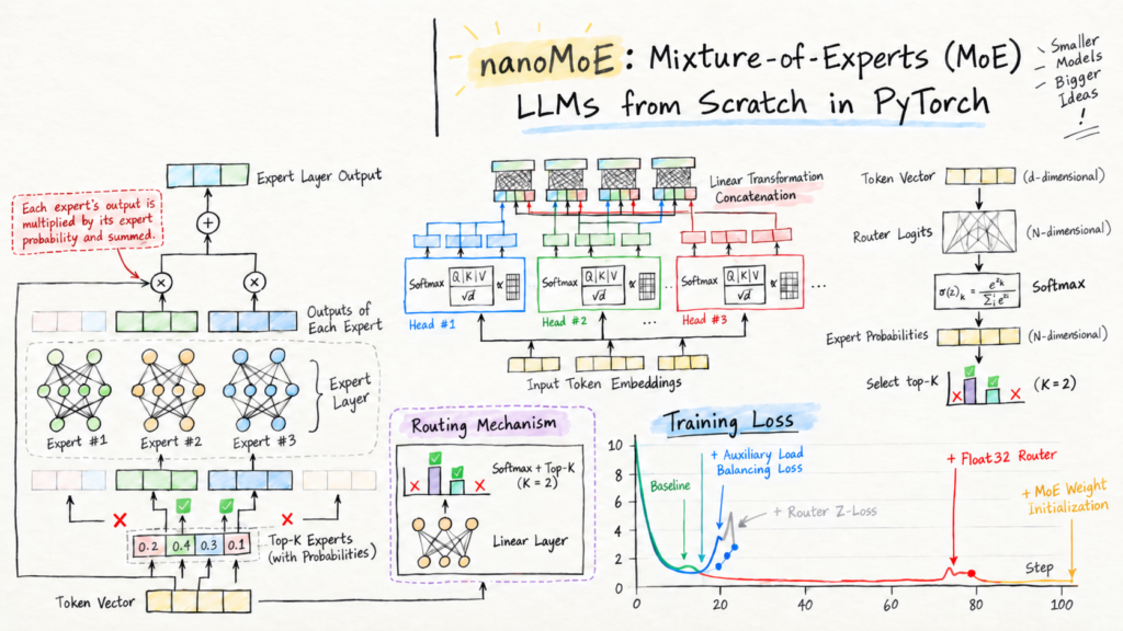
At a high level, MoE-based LLMs extend the standard decoder-only Transformer by introducing multiple expert networks and a routing mechanism that dynamically selects which experts should process each token. This creates a form of conditional computation: although an MoE model may contain a very large number of total parameters, only a fraction of those parameters are activated for any given token.
This sparsity is the key advantage of the MoE architecture. By activating only a subset of the model for each token, MoE models can substantially increase their total parameter count and representational capacity without requiring a proportional increase in computation. This makes it possible to build models with enormous capacity while keeping the computational cost of each forward pass comparatively manageable.
As MoE architectures become increasingly prominent in frontier language models, developing an intuitive and practical understanding of how they work is becoming increasingly important. In this post, we will take a step in that direction by building and pretraining a mid-sized MoE language model—nanoMoE—entirely from scratch in PyTorch.
The complete nanoMoE implementation is available in the accompanying repository, which is based on a fork of Andrej Karpathy’s nanoGPT and extended to support MoE architectures and pretraining. Rather than treating the MoE components as a black box, we will build the model incrementally from the ground up.
We will begin with the necessary background on Transformers and Mixture-of-Experts architectures. From there, we will implement each component of nanoMoE step by step, including the expert networks, routing mechanism, and sparse computation. Finally, we will bring everything together and run a complete pretraining experiment, resulting in a working MoE language model built entirely in PyTorch.
Basics of Decoder-Only Transformers
To understand Mixture-of-Experts (MoE) language models, we first need to establish a solid understanding of the standard architecture underlying most modern LLMs: the decoder-only Transformer.
The decoder-only Transformer is a simplified variant of the original encoder-decoder Transformer architecture introduced in and later popularized by models such as GPT. Although we have explored this architecture in detail in previous posts, it is worth revisiting the key components here, as a clear understanding of the standard Transformer will be essential for understanding how MoE architectures modify and extend it.
Throughout this section, we will use Andrej Karpathy’s nanoGPT implementation as a reference. nanoGPT provides a minimal yet fully functional implementation of a decoder-only Transformer, making it an ideal starting point for examining the architecture and understanding how its individual components fit together.
We will first walk through the core building blocks of a decoder-only Transformer and then use this foundation to understand how Mixture-of-Experts models introduce sparse, conditional computation into the architecture.
Original Architecture
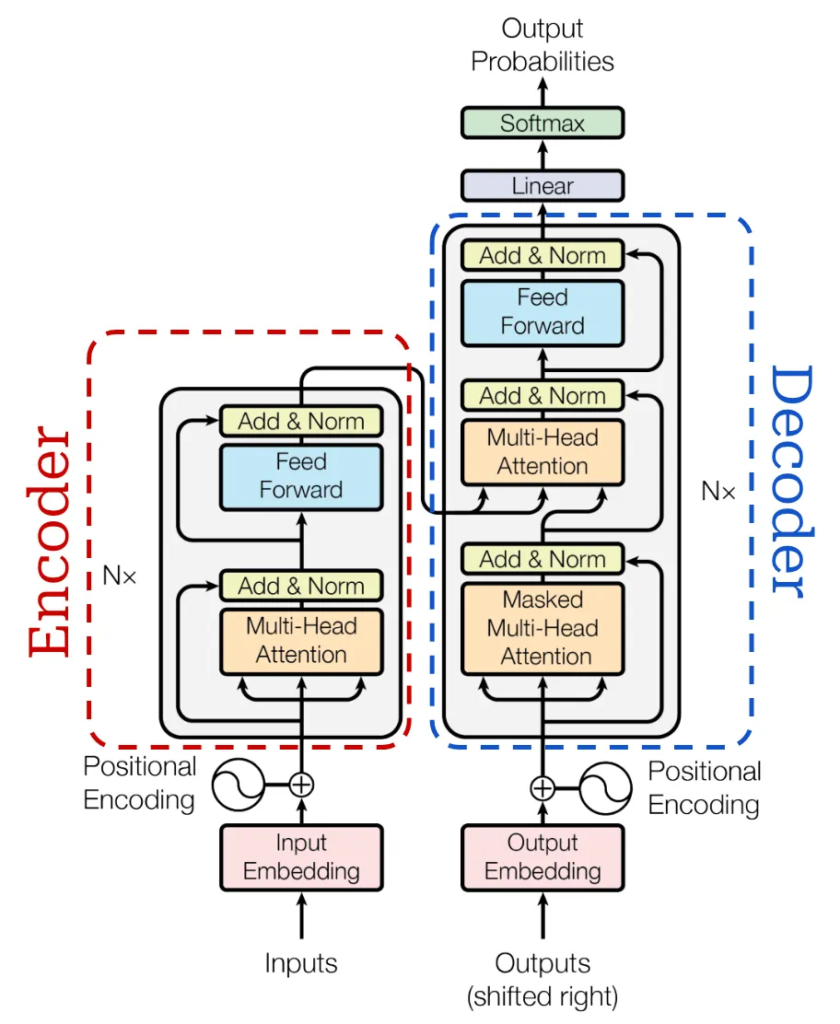
The Transformer architecture, originally introduced for machine translation in [1], consists of two primary components: an encoder and a decoder. We will not cover the complete encoder-decoder Transformer in detail here. However, a thorough and widely cited overview of the original architecture can be found here.
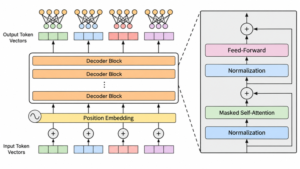
The decoder-only Transformer, which forms the foundation of most modern LLMs, simplifies this architecture by removing the encoder and retaining only the decoder. As the name suggests, the model consists entirely of a stack of decoder blocks.
In practice, each layer of a decoder-only Transformer contains two primary components:
- A masked self-attention layer, which allows each token to attend only to previous tokens in the sequence.
- A feed-forward network (FFN), which independently transforms the representations produced by the attention mechanism.
The complete decoder-only Transformer is constructed by stacking L such layers sequentially. While all layers share the same overall structure, each layer has its own independent set of learnable parameters. The output of one layer serves as the input to the next, allowing the model to progressively build richer representations of the input sequence.
A simplified view of this architecture is shown in the figure below.
Let’s now examine each component of the architecture individually to build a clearer understanding of how a decoder-only Transformer processes text. We will begin with the model’s input representation and then move through the main components of each Transformer layer—self-attention and the feed-forward network—before seeing how these pieces come together to form the complete model.
From Text to Tokens
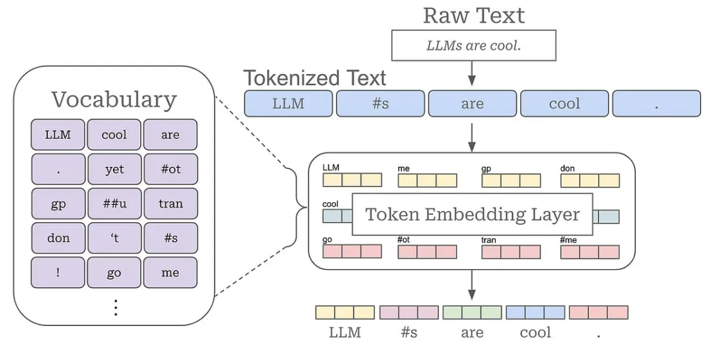
As we know, the input to an LLM is typically a sequence of text—a prompt written in natural language. However, the model does not directly operate on raw text. As illustrated in the figure above, the actual input to the Transformer is a sequence of token vectors.
This raises an important question: how do we transform a sequence of text into the numerical vectors that the model can process?
The answer involves two key steps: tokenization, which converts text into a sequence of discrete tokens, and embedding, which maps each token to a continuous vector representation. Let’s walk through these steps to understand how raw text is transformed into the input representation used by the Transformer.
Tokenization
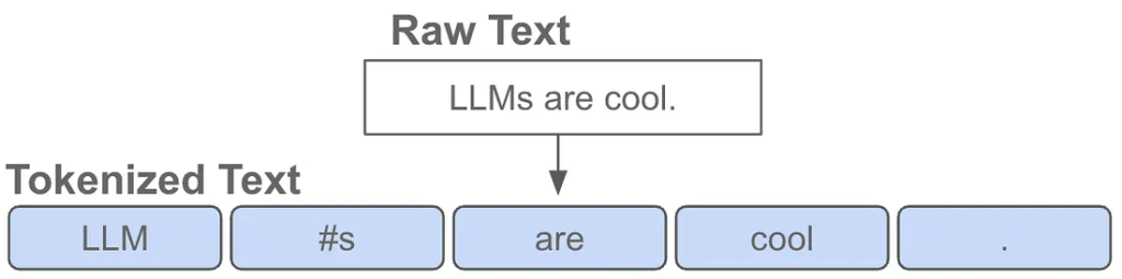
The first step in preparing text for an LLM is to convert the raw input—a sequence of characters—into a sequence of discrete tokens. This process is known as tokenization and is performed by the model’s tokenizer.
A tokenizer defines how text is split into manageable units that the model can represent and process. Depending on the tokenizer, these units may correspond to individual characters, words, subwords, or even bytes. Among the various approaches, Byte-Pair Encoding (BPE) tokenizers [2] are one of the most widely used methods in modern LLMs.These tokenizers take a sequence of raw text as input and break this text into a sequence of discrete tokens as shown in the figure above.
import torch
from transformers import AutoTokenizer

# load the llama-3.2 tokenizer
tokenizer = AutoTokenizer.from_pretrained('meta-llama/Llama-3.1-8B')

# raw text
text = "This raw text will be tokenized"

# create tokens using tokenizer
tokens = tokenizer.tokenize(text)
token_ids = tokenizer.convert_tokens_to_ids(tokens)
# token_ids = tokenizer.encode(text) # directly create token ids

# view the results
print("Original Text:", text)
print("Tokens:", tokens)
print("Token IDs:", token_ids)

# create token embedding layer
VOCABULARY_SIZE: int = 128000
EMBEDDING_DIM: int = 768
token_embedding_layer = torch.nn.Embedding(
        num_embeddings=VOCABULARY_SIZE,
        embedding_dim=EMBEDDING_DIM,
    )

# get token embeddings (IDs must be passed as a tensor, not a list)
token_emb = token_embedding_layer(torch.tensor(token_ids))
print(f'Token Embeddings Shape: {token_emb.shape}')
Tokenizers and Vocabulary
Modern LLM frameworks such as Hugging Face Transformers and torchtune provide convenient interfaces for working with tokenizers. OpenAI has also released tiktoken, a library for working with the tokenizers used by its GPT models.
At a high level, tokenization converts a raw text sequence into a list of discrete token units. For example:
Raw text:This raw text will be tokenized
Tokenized text:['This', 'Ġraw', 'Ġtext', 'Ġwill', 'Ġbe', 'Ġtoken', 'ized']
In this example, the Ġ character indicates that the token is preceded by whitespace. The exact convention used to represent whitespace or word boundaries depends on the tokenizer. Other tokenizers may use different special characters to represent word continuations. For example, a tokenizer might represent the final word as:
['token', '#ized']
The important point is that tokenization is tokenizer-dependent: different tokenizers can split the same piece of text into different sequences of tokens.
Vocabulary
Every LLM is trained using a specific tokenizer, although the same tokenizer can be shared across multiple models. Because the tokenizer defines a fixed set of tokens it can produce, the model also operates over a fixed set of discrete tokens. This collection is known as the model’s vocabulary.
The vocabulary determines the set of tokens the model can directly represent and process. Vocabulary sizes vary considerably across models and depend on factors such as the tokenizer design, training data, and language coverage. Multilingual models, for example, often require larger vocabularies to efficiently represent text across many languages.
For modern LLMs, vocabulary sizes ranging from roughly 64K to 256K tokens are relatively common. Once the vocabulary has been established, each token is assigned a unique integer ID, which allows the textual input to be converted into the numerical representation required by the Transformer.
Token IDs and Embeddings
Once the text has been tokenized, each token is mapped to a unique integer ID from the model’s vocabulary. For example, tokenizing our previous input produces the following sequence of token IDs:
[2028, 7257, 1495, 690, 387, 4037, 1534]
These integer IDs provide a compact way to represent the tokens, but they are not the representations that the Transformer operates on directly. Instead, each token ID is mapped to a dense numerical vector called a token embedding.
These embeddings are stored in an embedding layer, which can be viewed simply as a large matrix containing one vector for every token in the vocabulary. If the vocabulary contains V tokens and each embedding has dimensionality D, the embedding matrix has shape:
(V, D)
To obtain the embedding for a particular token, we simply use its token ID to index into this matrix and retrieve the corresponding row. Applying this lookup to every token in the input sequence transforms the sequence of integer token IDs into a sequence of dense vectors that can be passed into the Transformer.
In other words, the process can be summarized as:
Text → Tokens → Token IDs → Token Embeddings
This embedding lookup is the first step that converts discrete linguistic units into continuous numerical representations that the neural network can process.
Input Embeddings and Self-Attention
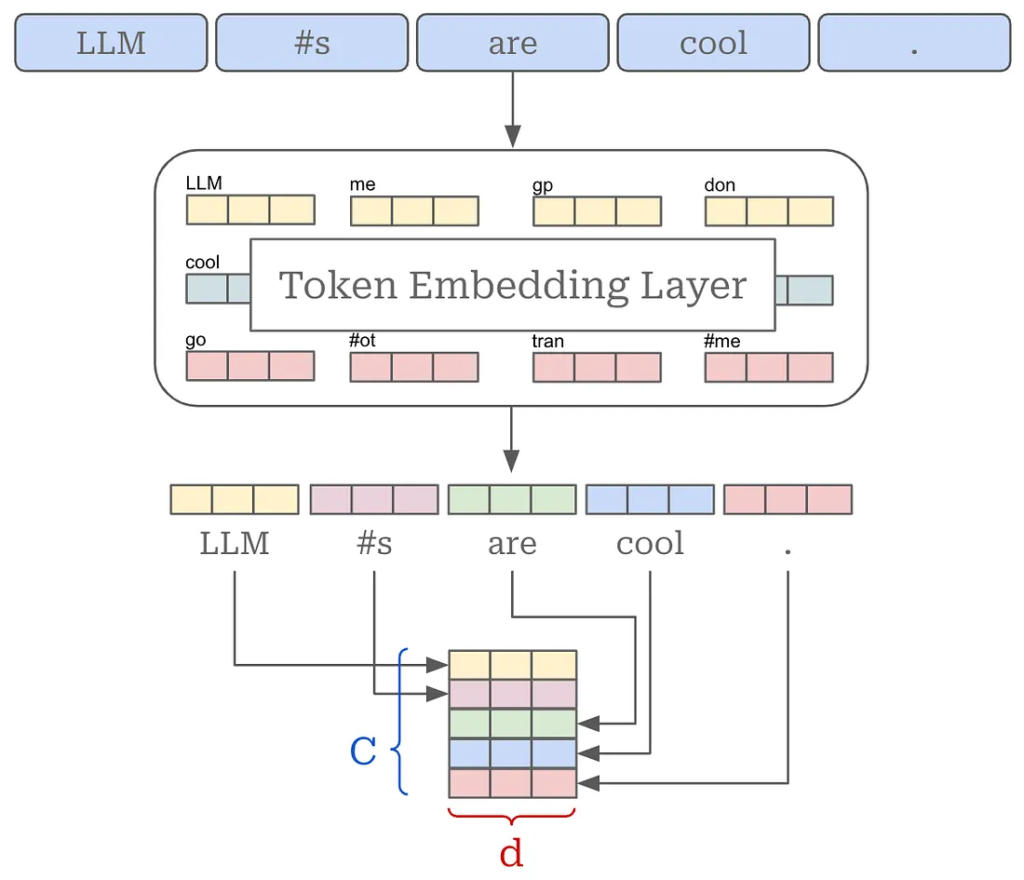
We now have a sequence of token embeddings, with one vector corresponding to each token in the input. By stacking these vectors together, we obtain a matrix that serves as the actual input to the Transformer, as illustrated above. In PyTorch, this conversion is handled automatically through the combination of the tokenizer and the model’s embedding layer.
For a single input sequence, the resulting token embedding matrix has shape [C, d], where:
- C is the number of tokens in the input sequence.
- d is the embedding dimension, i.e., the number of values used to represent each token.
In practice, LLMs process multiple sequences simultaneously in a batch. If the batch contains B sequences, the input becomes a three-dimensional tensor with shape [B, C, d].
The embedding dimension d is an important architectural hyperparameter because it determines the size of many of the model’s internal representations and directly influences the computational and memory requirements of the Transformer.
Before this input is passed through the Transformer, we also need to provide information about the position of each token in the sequence. Since self-attention itself does not inherently encode token order, a positional embedding is added to each token embedding. This allows the model to distinguish between tokens based not only on their content, but also on where they occur in the sequence.
(Masked and Multi-Headed) Self-Attention
With our input representation now constructed, we are ready to pass it into the decoder-only Transformer. As discussed earlier, the Transformer consists of a sequence of repeated blocks containing self-attention and feed-forward transformations, together with normalization operations.
We will begin by examining the self-attention mechanism, which is responsible for allowing each token to incorporate information from other tokens in the sequence.
What Is Self-Attention?
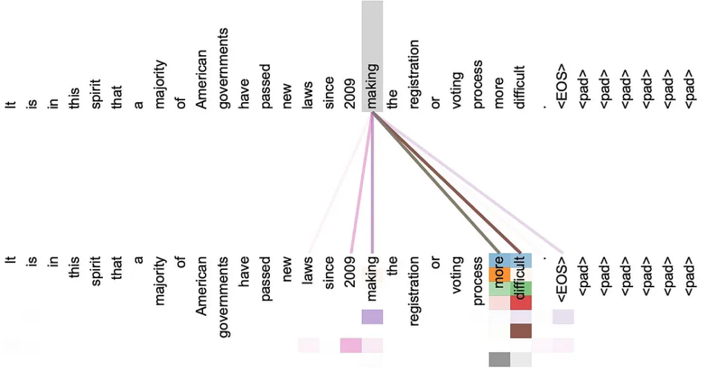
At its core, self-attention is a way for a model to understand each token by looking at the other tokens around it.
When we process a sentence, the meaning of a word often depends on the words surrounding it. Self-attention allows a model to figure out which other words are important for understanding the current word.
For example, consider a sentence containing the phrase:
“making the problem more difficult”
When the model processes the word making, it doesn’t look at that word in isolation. It can also pay attention to words such as more and difficult, because those words provide useful context for understanding what making means in this particular sentence.
So, you can think of self-attention as the model asking:
“Which other words should I pay attention to in order to better understand this word?”
The important part is that every token can look at all the other tokens in the sequence, including itself, and decide how much each one should contribute to its final representation.
The basic idea behind attention
A common way to describe attention is:
An attention mechanism takes a query and compares it with a collection of keys. These comparisons determine how much attention should be given to the corresponding values.
In simpler terms:
Query → What am I looking for?
Key → What information do I contain?
Value → What information should I actually pass along?
The model compares a query with different keys, calculates how relevant they are, and then combines the corresponding values using those relevance scores.
Scaled Dot-Product Attention
Now let’s look at how this works mathematically.
Suppose our input sequence contains C tokens, and each token is represented using d features. We can represent the entire sequence as a matrix with the shape:
[C, d]
For simplicity, let’s assume we’re processing one sequence at a time rather than a batch of sequences.
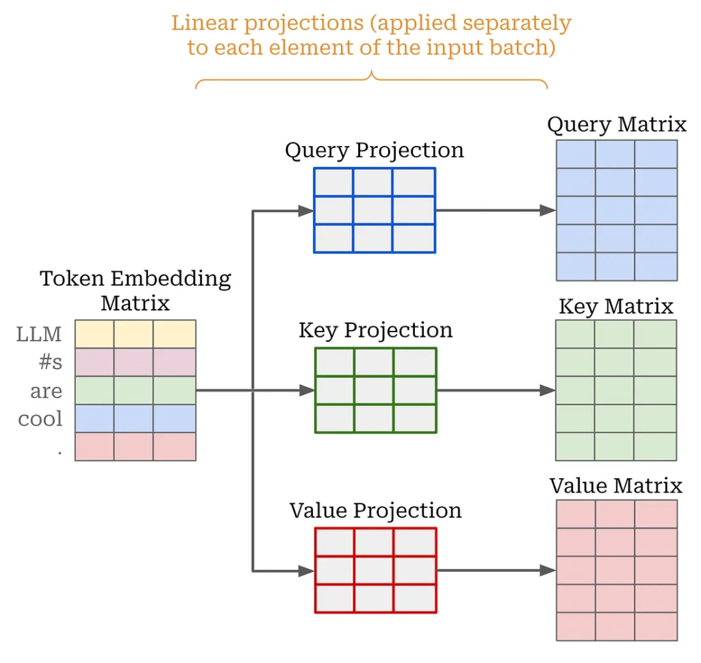
The first step is to take our input token representations and pass them through three separate linear transformations.
These three transformations produce three new representations:
- Query (Q) — represents what each token is looking for.
- Key (K) — represents what information each token can provide for matching.
- Value (V) — contains the actual information that will be passed forward.
So, instead of working directly with the original token representations, self-attention creates three different views of the same input:
Input → Query, Key, Value
The model then compares the queries with the keys to determine which tokens are most relevant to one another. Those relevance scores are used to combine the value vectors and produce the final attention-aware representation.
This is the core idea behind scaled dot-product attention, which forms the foundation of the attention mechanism used in modern Transformer models.
Why Do We Call Them Query, Key, and Value?
At first, the names query, key, and value can feel a little arbitrary. But they actually come from an idea that has been used for a long time in information retrieval and search systems.
A simple way to understand the three terms is to think about how a search works.
- Query (Q): This is what we’re looking for. In self-attention, the query represents the current token and helps the model find other tokens that are relevant to it.
- Key (K): Think of the key as an identifier or index for each token. The model compares a query with different keys to figure out which tokens are the most relevant.
- Value (V): The value contains the actual information associated with a token. Once the model determines that a particular key is relevant to the query, the corresponding value contributes to the final representation.
A simple analogy is a search engine:
Query → Search for relevant Keys → Retrieve their Values
That’s essentially the idea behind attention.
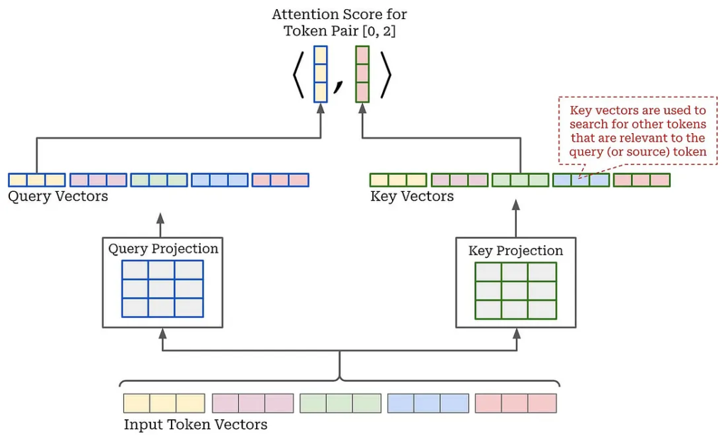
Computing Attention Scores
Once we’ve created the Query, Key, and Value representations, the next step is to figure out how much attention each token should give to the other tokens.
For every pair of tokens (i, j) in the sequence, we calculate an attention score a[i, j].
This score tells us how relevant token j is when we’re trying to understand token i.
You can think of it as the model asking:
“How important is token
jfor understanding tokeni?”
A higher score means the two tokens are more closely related in the current context, while a lower score means the relationship is weaker.
The attention scores are calculated using the query and key vectors.
For token i, we take its query vector and compare it with the key vector of token j. This comparison is done using a dot product:
Query of token i · Key of token j
If the resulting vectors point in similar directions, their dot product will generally be larger, indicating a stronger relationship. If they are less aligned, the score will be smaller.
In other words:
Query tells us what we’re looking for.
Key tells us what each token offers for matching.
The dot product tells us how well they match.
These scores are then processed and normalized to determine how much attention should ultimately be given to each token.
Computing All Attention Scores at Once
Instead of calculating the attention score for every pair of tokens one at a time, we can do the whole calculation efficiently using matrix multiplication.
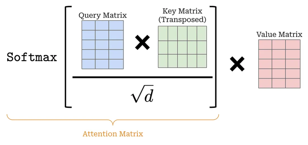
First, we stack all of our query vectors into a Query matrix (Q) and all of our key vectors into a Key matrix (K).
We then multiply the Query matrix by the transpose of the Key matrix:
Q × Kᵀ
The result is a square matrix with the shape:
[C, C]
This is called the attention matrix.
Why is its size [C, C]?
Because we have C tokens, and we want to know how strongly every token relates to every other token. Each row represents one token asking, “Which other tokens are important to me?”, while each column represents the token being considered as a potential source of information.
Scaling the Scores
The raw values produced by Q × Kᵀ can become quite large, especially as the dimension d increases. To keep these values under control and make training more stable, we scale the entire attention matrix by dividing it by:
√d
So the operation becomes:
QKᵀ / √d
This small step is important because it prevents the attention scores from becoming excessively large, which can otherwise make the softmax function behave poorly during training.
Applying Softmax
Next, we apply the softmax function to each row of the scaled attention matrix.
Softmax converts the raw attention scores into probabilities. After this step:
- Every value is positive.
- The values in each row add up to 1.
- Larger values indicate that the model is assigning more attention to that particular token.
For example, if one row contains:
[0.05, 0.10, 0.70, 0.15]
the third token receives the most attention because it has the highest probability.
So, the i-th row of the attention matrix tells us how the i-th token distributes its attention across every token in the sequence.
Putting everything together, the process looks like this:
Q and K → QKᵀ → Scale by √d → Softmax → Attention weights
These attention weights are then used in the next step to determine how much information should be gathered from the Value (V) vectors.
Computing the Output
Once we have calculated the attention scores, getting the final output of self-attention is actually pretty straightforward.
Remember that the attention scores tell us how much each token should pay attention to every other token. We can now use those scores to combine the information stored in the Value (V) vectors.
For each token, we take a weighted combination of all the value vectors. The attention scores determine the weights.
In matrix form, this is simply:
Attention × V
where:
- Attention contains the normalized attention weights.
- V contains the value vectors.
- The result is the new representation of every token after incorporating information from the rest of the sequence.
An important property of self-attention is that it preserves the sequence dimensions.
If our input contains C tokens and each token is represented using d dimensions, the output will also contain C tokens, each represented using d dimensions.
So, in simple terms:
Input: [C, d]
Output: [C, d]
The vectors have been transformed and enriched with information from other tokens, but the overall shape remains the same.
Masked Self-Attention
So far, we’ve been talking about vanilla self-attention, also known as bidirectional self-attention.
In this setup, every token can look at every other token in the sequence. A token can use information from both the tokens before it and the tokens after it.
That’s useful for models such as encoder-based Transformers, but it isn’t appropriate for decoder-only models that generate text one token at a time.
Imagine the model is generating:
“The cat is sitting on the…”
When predicting the next token, the model should only have access to the information that has already been generated. It shouldn’t be able to look ahead and see the words that come later.
This is where masked self-attention comes in.
Masked self-attention prevents each token from attending to tokens that appear after it in the sequence.
For example:
| Token | Can attend to |
|---|---|
The | The |
cat | The, cat |
is | The, cat, is |
sitting | The, cat, is, sitting |
The first token can only see itself. The second token can see the first and second tokens. The third token can see the first three tokens, and so on.
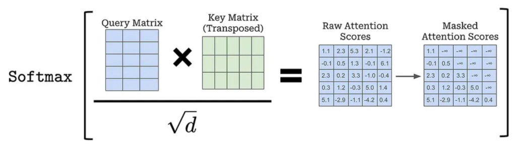
The future tokens are effectively masked out before the softmax operation, so their attention weights become zero.
This creates a triangular attention pattern where each token can only attend to itself and the tokens that came before it.
That’s the key idea behind causal or masked self-attention, which allows decoder-only Transformers to generate text from left to right without getting access to future information.
Computing output. Once we have the attention scores, deriving the output of self-attention is easy. The output for each token is simply a weighted combination of value vectors, where the weights are given by the attention scores. To compute this output, we simply multiply the attention matrix by the value matrix as shown above. Notably, self-attention preserves the size of its input — a transformed, d-dimensional output vector is produced for each token vector within the input.
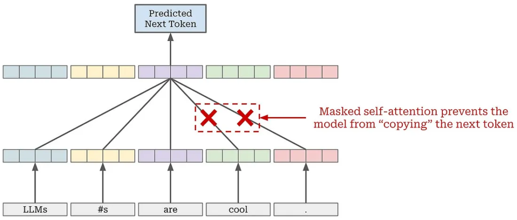
Masked self-attention. So far, the formulation we have learned is for vanilla (or bidirectional self-attention). As mentioned previously, however, decoder-only transformers use masked self-attention, which modifies the underlying attention pattern by “masking out” tokens that come after each token in the sequence. Each token can only consider tokens that come before it — following tokens are masked.
Example: Masked Self-Attention
Let’s make masked self-attention more concrete with a simple example.
Suppose our input sequence is:
["LLM", "#s", "are", "cool", "."]
Now, let’s focus on the token "are".
With regular self-attention, "are" would be allowed to look at every token in the sequence:
LLM#sarecool.
This means "are" could use information from tokens that appear both before and after it.
But that’s not allowed in masked self-attention.
Because "are" is the third token, it can only attend to the tokens that have already appeared:
["LLM", "#s", "are"]
The tokens that come after it:
["cool", "."]
are considered future tokens and are therefore masked.
How does the masking work?
The model calculates the attention scores as usual, but before applying softmax, it sets the scores for future tokens to negative infinity (-∞).
Conceptually, the attention scores for "are" might look something like this:
| Token | Attention score |
|---|---|
LLM | 1.2 |
#s | 0.8 |
are | 1.5 |
cool | -∞ |
. | -∞ |
When softmax is applied, the -∞ values become zero probability.
So the resulting attention distribution might look like:
[0.30, 0.20, 0.50, 0.00, 0.00]
The exact numbers will depend on the model’s learned representations, but the important part is:
cool → 0. → 0
The model is therefore prevented from looking ahead.
This simple masking mechanism is what makes causal self-attention possible. During text generation, the model can use everything it has already seen, but it cannot access tokens that haven’t been generated yet.
In short:
Masked self-attention lets a token look backward and at itself, but never forward.
That’s essential for autoregressive language models because it prevents the model from “cheating” by seeing the answer before predicting it.
Attention Heads
So far, we have looked at attention as a single operation where the attention scores are normalized using softmax across the sequence. While this works well, there is a limitation: the resulting probability distribution can become heavily concentrated on one or a few tokens.
This can make it difficult for the model to pay attention to several different positions in the sequence at the same time.
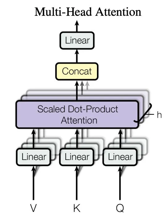
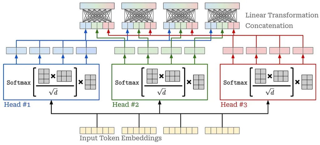
A common solution is multi-head attention. Instead of performing attention once, we run several attention operations, called heads, in parallel.
Each attention head works independently, but there are two important differences:
- Each head has its own key, query, and value projections. This allows different heads to learn and focus on different relationships between tokens.
- The key, query, and value vectors are smaller in each head. Reducing their dimensionality keeps the overall computational cost manageable.
More specifically, if the original vector dimension is d and we use H attention heads, each head typically works with vectors of dimension:
d // H
This way, even though we are running multiple attention heads in parallel, the overall computational cost remains roughly comparable to using a single attention operation with the full dimension.
The key idea is simple: instead of asking one attention mechanism to capture every relationship in the sequence, we let multiple smaller attention heads learn different relationships simultaneously.
Combining the Outputs of Attention Heads
At this point, we have multiple attention heads running in parallel, with each head performing its own self-attention operation. But we still need to combine their outputs into a single representation that can be passed to the next layer.
There are several ways we could combine the outputs, such as averaging them, concatenating them, or passing them through another projection layer.
In the standard implementation of multi-head self-attention, we use two simple steps:
- Concatenate the outputs from all attention heads.
- Apply a linear projection to the concatenated result.
Each attention head produces token representations with a dimension of d // H, where d is the original embedding dimension and H is the number of attention heads.
When we concatenate the outputs from all H heads, the dimensions add up:
H × (d // H) = d
So, the final output has the same dimension d as the original input.
This is an important design choice: multi-head attention allows the model to learn different relationships in parallel without changing the overall size of the representation.
"""
Source: https://github.com/karpathy/nanoGPT/blob/master/model.py
"""

import math
import torch
from torch import nn
import torch.nn.functional as F

class CausalSelfAttention(nn.Module):

    def __init__(
            self,
            d,
            H,
            T,
            bias=False,
            dropout=0.2,
        ):
    """
    Arguments:
        d: size of embedding dimension
        H: number of attention heads
        T: maximum length of input sequences (in tokens)
        bias: whether or not to use bias in linear layers
        dropout: probability of dropout
        """
        super().__init__()
        assert d % H == 0

        # key, query, value projections for all heads, but in a batch
        # output is 3X the dimension because it includes key, query and value
        self.c_attn = nn.Linear(d, 3*d, bias=bias)

        # projection of concatenated attention head outputs
        self.c_proj = nn.Linear(d, d, bias=bias)

        # dropout modules
        self.attn_dropout = nn.Dropout(dropout)
        self.resid_dropout = nn.Dropout(dropout)
        self.H = H
        self.d = d

        # causal mask to ensure that attention is only applied to
        # the left in the input sequence
        self.register_buffer("mask", torch.tril(torch.ones(T, T))
            .view(1, 1, T, T))

        def forward(self, x):
            B, T, _ = x.size() # batch size, sequence length, embedding dimensionality

            # compute query, key, and value vectors for all heads in batch
            # split the output into separate query, key, and value tensors
            q, k, v = self.c_attn(x).split(self.d, dim=2) # [B, T, d]

            # reshape tensor into sequences of smaller token vectors for each head
            k = k.view(B, T, self.H, self.d // self.H).transpose(1, 2) # [B, H, T, d // H]
            q = q.view(B, T, self.H, self.d // self.H).transpose(1, 2)
            v = v.view(B, T, self.H, self.d // self.H).transpose(1, 2)

            # compute the attention matrix, perform masking, and apply dropout
            att = (q @ k.transpose(-2, -1)) * (1.0 / math.sqrt(k.size(-1))) # [B, H, T, T]
            att = att.masked_fill(self.mask[:,:,:T,:T] == 0, float('-inf'))
            att = F.softmax(att, dim=-1)
            att = self.attn_dropout(att)

            # compute output vectors for each token
            y = att @ v # [B, H, T, d // H]

            # concatenate outputs from each attention head and linearly project
            y = y.transpose(1, 2).contiguous().view(B, T, self.d)
            y = self.resid_dropout(self.c_proj(y))
            return y
Full Implementation
Now let’s put everything together and look at the complete implementation of masked multi-head self-attention.
So far, we have considered a single input sequence with a shape of [C, d]. In a real model, we usually process multiple sequences at once, so the input has the shape [B, C, d], where:
B= batch sizeC= sequence lengthd= embedding dimension
The implementation above brings together all the steps we have discussed:
- Lines 52–59: We compute the key, query, and value projections for all attention heads. A single linear projection is used initially, after which the results are split and reshaped so that each attention head can operate independently.
- Lines 62–65: We calculate the attention scores, apply the causal mask so that each token can only attend to the appropriate previous tokens, and then use softmax to convert the scores into attention weights.
- Line 68: We multiply the attention weights by the value matrix to produce the output representation for each attention head.
- Lines 71–72: We concatenate the outputs from all attention heads and pass the combined representation through a linear projection to produce the final output.
The PyTorch code may look a little complicated because it relies on matrix operations, reshaping, and tensor manipulation. But underneath all of that, the implementation is simply putting together the exact steps we have already covered:
Project → Split into heads → Calculate attention → Apply mask → Softmax → Combine values → Concatenate heads → Project the output.
So, while the code involves some sophisticated tensor operations, the underlying idea is still the same masked multi-head self-attention mechanism we described earlier.
Feed-Forward Transformation
Feed-Forward Network
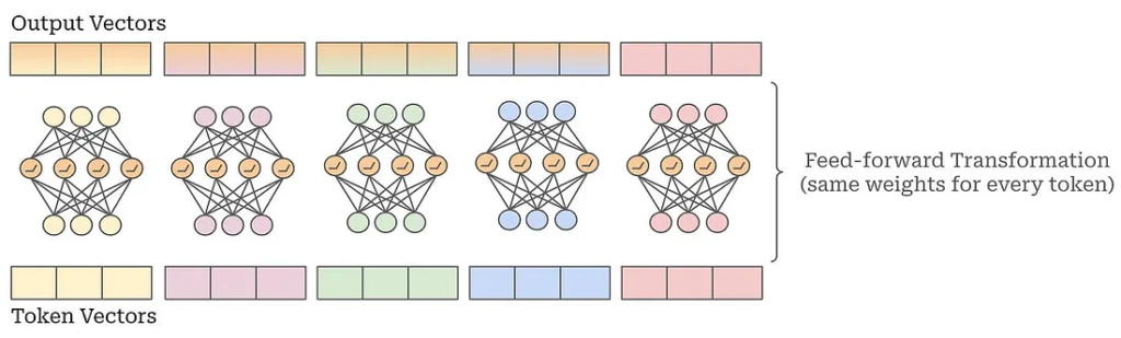
Along with masked self-attention, every Transformer block also contains a pointwise feed-forward network (FFN).
The idea is fairly simple: after the attention mechanism has gathered information from different tokens, the feed-forward network processes each token independently using the same neural network.
Typically, this feed-forward network consists of two linear layers with a non-linear activation function between them. Common activation functions include ReLU, GeLU, and SwiGLU.
The structure looks like this:
Input → Linear Layer → Activation → Linear Layer → Output
An important detail is that the hidden layer is usually larger than the original token embedding dimension. A common design is to expand the dimension by around 4× before projecting it back to the original size.
For example, if the token embedding dimension is d = 768, the hidden layer might use a dimension of 3072.
In PyTorch, implementing this type of feed-forward network is straightforward using the Linear module along with the desired activation function.
The key point to remember is that self-attention allows tokens to interact with each other, while the feed-forward network transforms each token’s representation independently. Together, these components form the core computation inside a Transformer block.
"""
Source: https://github.com/karpathy/nanoGPT/blob/master/model.py
"""

from torch import nn

class MLP(nn.Module):

    def __init__(
            self,
            d,
            bias=False,
            dropout=0.2
        ):
    """
    Arguments:
        d: size of embedding dimension
        bias: whether or not to use bias in linear layers
        dropout: probability of dropout
        """

        super().__init__()
        self.c_fc = nn.Linear(d, 4 * d, bias=bias)
        self.gelu = nn.GELU()
        self.c_proj = nn.Linear(4 * d, d, bias=bias)
        self.dropout = nn.Dropout(dropout)

        def forward(self, x):
            x = self.c_fc(x)
            x = self.gelu(x)
            x = self.c_proj(x)
            x = self.dropout(x)
            return x
Decoder-Only Transformer Block
Decoder-Only Transformer Block
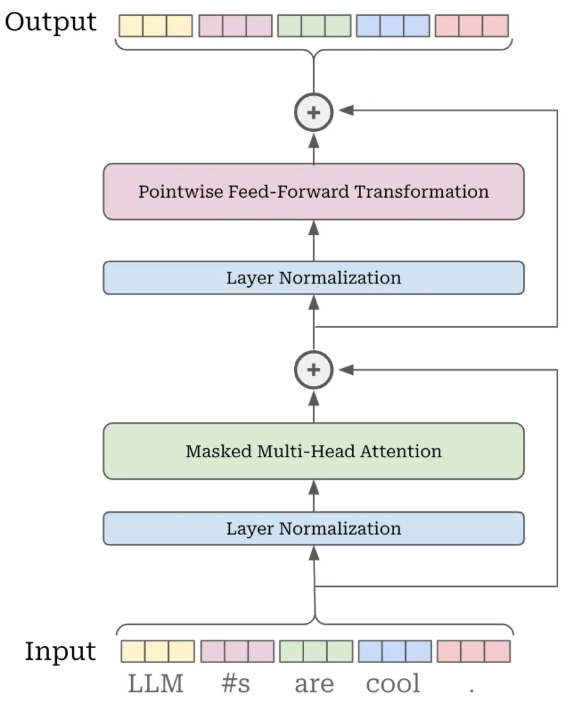
Now we can bring the pieces together to build a decoder-only Transformer block.
A typical block combines the two main components we have already discussed:
- Masked multi-head self-attention — allows each token to interact with the relevant tokens that come before it.
- Feed-forward network (FFN) — processes each token’s representation independently.
In addition to these two components, Transformer blocks also use normalization layers and residual connections to make the network easier to train and more stable.
A simplified view of the block is:
Input → Normalization → Masked Self-Attention → Residual Connection → Normalization → Feed-Forward Network → Residual Connection → Output
The exact ordering of normalization and other components can vary between Transformer architectures, but the core idea remains the same.
What is a Residual Connection?
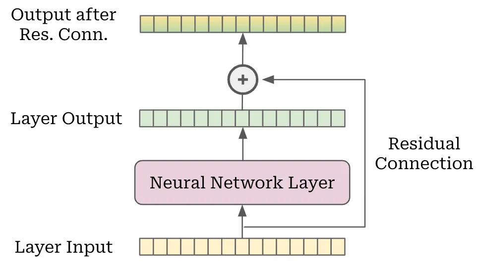
A residual connection provides a shortcut around a neural network layer. Instead of passing only the layer’s output to the next layer, we add the original input back to that output:
Output = Layer(Input) + Input
This allows information from earlier layers to flow directly through the network rather than being transformed at every step.
Residual connections are particularly important in deep Transformer models because they help preserve information and make it easier for the model to learn as the number of layers increases.
So, at a high level, a decoder-only Transformer block repeatedly performs two things:
Self-attention → Understand relationships between tokens
Feed-forward network → Transform each token’s representation
Residual connections and normalization are then used around these components to help the entire network train effectively.
Why Residual Connections Matter
Residual connections are a common technique used throughout deep learning and aren’t limited to Transformer models. They can be added around many different types of neural network layers.
The main purpose of a residual connection is to make deep networks easier and more stable to train.
Without a residual connection, the gradient has to pass through every layer during backpropagation. As the network gets deeper, this can lead to problems such as vanishing or exploding gradients, making it difficult for earlier layers to learn effectively.
A residual connection provides a shortcut that allows information — and importantly, gradients — to flow more directly through the network.
Conceptually, instead of:
Input → Layer → Output
we use:
Input → Layer → + Input → Output
In other words:
Output = Layer(Input) + Input
This seemingly simple addition can make a significant difference when training deep neural networks.
The key idea is that the network doesn’t have to learn an entirely new representation at every layer. It can preserve useful information from the input and learn only the additional transformation, or “residual,” that needs to be applied.
This is one of the reasons residual connections are so important in modern architectures such as Transformers.
Layer Normalization
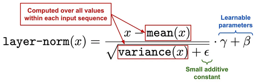
Another important component used in Transformer models is normalization. Normalizing the inputs or outputs of neural network layers can make training more stable and help the model converge more effectively.
There are several types of normalization techniques, but Layer Normalization (LayerNorm) is the one most commonly associated with Transformers and LLMs.
Layer normalization can be thought of as having two main steps:
- Normalize the values — the activations are normalized so that they have a more controlled distribution.
- Apply a learnable transformation — instead of using the normalized values directly, the model scales them using a learnable weight and shifts them using a learnable bias.
Conceptually:
Output = Normalized(Input) × Weight + Bias
The weight and bias are learnable parameters, meaning the model adjusts them during training along with all its other parameters.
This gives the model some flexibility: normalization keeps the activations well-behaved, while the learnable scale and shift allow the network to adjust the normalized representation when necessary.
In PyTorch, LayerNorm is already available through the LayerNorm module, making it straightforward to add normalization to a Transformer block.
In short, residual connections help information and gradients flow through deep networks, while layer normalization helps keep the activations stable during training. Together, they play an important role in making modern Transformer architectures practical to train.
"""
Source: https://github.com/karpathy/nanoGPT/blob/master/model.py
"""

from torch import nn

class Block(nn.Module):
    def __init__(
            self,
            d,
            H,
            T,
            bias=False,
            dropout=0.2,
        ):
    """
    Arguments:
        d: size of embedding dimension
        H: number of attention heads
        T: maximum length of input sequences (in tokens)
        bias: whether or not to use bias in linear layers
        dropout: probability of dropout
        """

        super().__init__()
        self.ln_1 = nn.LayerNorm(d)
        self.attn = CausalSelfAttention(d, H, T, bias, dropout)
        self.ln_2 = nn.LayerNorm(d)
        self.ffnn = MLP(d, bias, dropout)

        def forward(self, x):
            x = x + self.attn(self.ln_1(x))
            x = x + self.ffnn(self.ln_2(x))
            return x
Block Implementation
Now we can put everything we’ve learned together and implement a complete decoder-only Transformer block.
Since we’ve already built the masked multi-head self-attention and feed-forward network components, the block itself becomes much simpler. We can simply combine these existing modules with the residual connections and layer normalization we discussed earlier.
This modular approach is one of the strengths of deep learning frameworks such as PyTorch. Instead of implementing everything from scratch in one large piece of code, we can build smaller components and then combine them to form a complete Transformer block.
Decoder-Only Transformer Architecture
Once we understand how the input flows through a decoder-only Transformer block, the overall architecture is quite straightforward.
We simply stack the same Transformer block L times.
Each block receives an input tensor with the shape:
[B, C, d]
where:
B= batch sizeC= sequence lengthd= model or embedding dimension
An important point is that the dimensions remain unchanged as the representation moves through the Transformer blocks.
So, if the input to the first block has the shape [B, C, d], its output has the same shape. That output then becomes the input to the next block, and this continues through all L layers.
Conceptually:
Input → Block 1 → Block 2 → Block 3 → … → Block L → Output
Even though the shape stays the same, the representation becomes increasingly richer as it passes through each block. Each layer can refine the information by combining self-attention, feed-forward transformations, normalization, and residual connections.
Therefore, the output of the final decoder-only Transformer block is still a tensor of shape:
[B, C, d]
This simple idea — repeating the same Transformer block multiple times while preserving the representation size — forms the foundation of decoder-only architectures such as GPT-style language models.
Full GPT-Style Decoder-Only Transformer
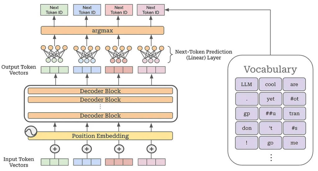
Now we can bring all the pieces together to build a complete GPT-style decoder-only Transformer.
The architecture consists of several key components:
- Token embedding layer — converts each input token ID into a learned vector representation.
- Positional embedding layer — adds information about the position of each token in the sequence.
LTransformer blocks — repeatedly process the representations using masked self-attention, feed-forward networks, residual connections, and layer normalization.- Final layer normalization — normalizes the representation produced by the last Transformer block.
- Linear output layer — converts the final token representations into scores for every token in the vocabulary.
The model starts with a sequence of token IDs with the shape:
[B, C]
where:
B= batch sizeC= sequence length
These token IDs first pass through the token and positional embedding layers. The resulting representations are then passed through all L Transformer blocks.
Finally, the output is normalized and passed through a linear layer to produce logits, which represent the model’s scores for the possible next tokens.
The overall flow can be summarized as:
Token IDs → Token Embeddings + Position Embeddings → Transformer Blocks × L → LayerNorm → Linear Layer → Next-Token Logits
During generation, the model uses these logits to determine which token should come next. The selected token is then added to the sequence, and the process is repeated to generate the rest of the text.
So, despite the complexity of the individual components, the overall GPT-style architecture follows a fairly simple pipeline:
Take token IDs → build their representations → repeatedly transform them with Transformer blocks → predict the next token.
That’s the core architecture behind decoder-only language models such as GPT.
"""
Source: https://github.com/karpathy/nanoGPT/blob/master/model.py
"""

import torch
from torch import nn
import torch.nn.functional as F

class GPT(nn.Module):

    def __init__(self,
    d,
    H,
    C,
    V,
    layers,
    bias=False,
    dropout=0.2,
):
"""
Arguments:
    d: size of embedding dimension
    H: number of attention heads
    C: maximum length of input sequences (in tokens)
    V: size of the token vocabulary
    layers: number of decoder-only blocks
    bias: whether or not to use bias in linear layers
    dropout: probability of dropout
    """

    super().__init__()
    self.transformer = nn.ModuleDict(dict(
            wte=nn.Embedding(V, d), # token embeddings
            wpe=nn.Embedding(C, d), # position embeddings
            drop=nn.Dropout(dropout),
            blocks=nn.ModuleList([Block(d, H, C, bias, dropout) for _ in range(layers)]),
            ln_f=nn.LayerNorm(d),
            head=nn.Linear(d, V, bias=bias),
        ))

def forward(self, idx, targets=None):
    # idx is a [B, C] matrix of token indices
    # targets is a [B, C] matrix of target (next) token indices
    device = idx.device
    _, C = idx.size() # [B, C]
    pos = torch.arange(0, C, dtype=torch.long, device=device)

    # generate token and position embeddings
    tok_emb = self.transformer.wte(idx) # [B, C, d]
    pos_emb = self.transformer.wpe(pos) # [C, d]
    x = self.transformer.drop(tok_emb + pos_emb)

    # pass through all decoder-only blocks
    for block in self.transformer.blocks:
        x = block(x)
        x = self.transformer.ln_f(x) # final layer norm

        if targets is not None:
            # compute the loss if we are given targets
            logits = self.transformer.head(x)
            loss = F.cross_entropy(
                    logits.view(-1, logits.size(-1)),
                    targets.view(-1),
                    ignore_index=-1,
                )
        else:
            # only look at last token if performing inference
            logits = self.transformer.head(x[:, [-1], :])
            loss = None

            return logits, loss
Generating Output: Decoding
LLMs are trained primarily for next-token prediction. In simple terms, the model looks at the tokens it has received so far and predicts what token should come next.
After passing the input through the decoder-only Transformer, the model produces an output vector for every token in the sequence. To predict the next token, we focus on the output vector corresponding to the last token.
The process is straightforward:
- Take the output vector for the last token in the sequence.
- Pass it through a linear layer that maps the vector to the size of the model’s vocabulary. This produces a score, or logit, for every possible token.
- Select the next token based on these scores. With greedy decoding, we simply use
argmaxto select the token with the highest score.
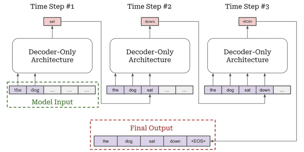
Once we have the next token, we append it to the existing sequence and run the model again.
For example:
Prompt → Model → Predict next token → Add token → Model → Predict next token → Add token → …
This process continues until the model reaches a stopping condition, such as an end-of-sequence token or a predefined maximum length.
This is called autoregressive decoding because each newly generated token becomes part of the input used to predict the following token.
So, at a high level, generating text with an LLM is simply a repeated loop:
Input tokens → Transformer → Last-token representation → Vocabulary scores → Next token → Add to sequence → Repeat
One important detail is that argmax represents greedy decoding. Modern LLMs can also use strategies such as temperature sampling, top-k sampling, or top-p (nucleus) sampling to choose the next token, which can produce more varied outputs.
Why Do LLMs Use the Decoder?
Now that we understand how a decoder-only Transformer works, a natural question comes up:
Why do modern LLMs primarily use the decoder instead of the full encoder-decoder architecture?
The main difference between the Transformer encoder and decoder comes down to how attention works.
An encoder uses bidirectional self-attention. This means that when processing a token, the model can look at tokens both before and after it in the sequence.
For example, when processing:
The cat sat on the mat
the encoder can use information from the entire sequence when representing the word cat, including tokens that appear later.
A decoder, on the other hand, uses masked self-attention. The attention mask prevents a token from looking at tokens that come after it.
So, when generating text, the model can only use information that is already available:
The → The cat → The cat sat → The cat sat on → ...
This restriction is important for next-token prediction. During training, the model learns to predict the next token without being able to see the answer ahead of time.
For example:
The cat sat on the ___
The model can use everything before the blank, but it cannot look at the actual next token while making its prediction.
This makes the decoder architecture a natural fit for autoregressive language generation.
In simple terms:
Encoder → Can look both left and right → Good for understanding the full context
Decoder → Can only look to the left → Good for predicting what comes next
Since GPT-style LLMs are trained primarily as next-token predictors, masked self-attention provides exactly the behavior they need for generating text one token at a time.
Why Masked Attention Works
Masked self-attention is one of the key reasons decoder-only Transformers work so well for next-token prediction.
During training, each token must predict what comes next. If a token were allowed to attend to tokens that appear later in the sequence, the model could simply look at the answer instead of actually learning how to predict it.
For example, consider:
The cat is sitting on the ___
The model should predict the next token using only the information available before it. If it could see the tokens that come after the blank, it could potentially learn to copy the answer rather than learning meaningful patterns in the language.
The causal mask prevents this by blocking access to future tokens.
As a result, the model is forced to learn relationships and patterns from the tokens that have already appeared. This makes masked self-attention a natural fit for autoregressive language models.
Creating a Mixture-of-Experts (MoE) Model
Now that we have a good understanding of decoder-only Transformers, we can take the next step and introduce a Mixture-of-Experts (MoE) architecture.
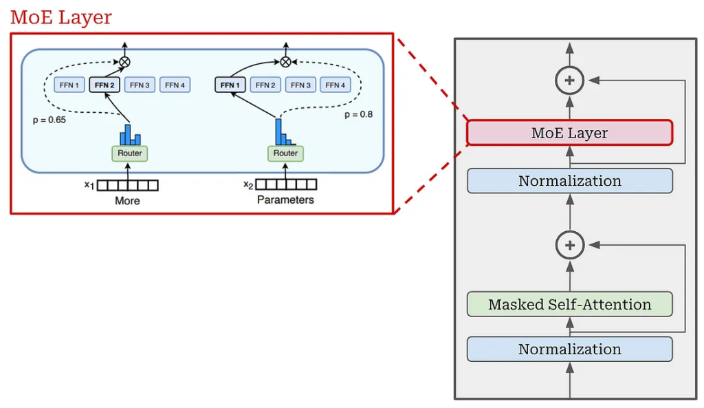
An MoE model keeps the basic decoder-only Transformer structure, but changes how the feed-forward network works.
The main idea behind MoE is that instead of using the exact same parameters for every input token, the model has multiple specialized networks, called experts, and selectively uses some of them for each token.
This creates a sparsely activated model: the model can contain a very large number of parameters, while only a subset of those parameters are actually used for a particular input.
The overall Transformer architecture remains largely the same. The main modification happens inside the feed-forward component of each Transformer block.
Expert Layers
In a standard decoder-only Transformer, each block contains a single feed-forward network that processes every token.
With MoE, we replace that single feed-forward network with multiple independent feed-forward networks.
Each network has its own set of weights and can learn different patterns or transformations. These individual networks are called experts.
For example, if an MoE layer contains N experts, we can represent them as:
E₁, E₂, E₃, ..., Eₙ
Instead of sending every token through the same feed-forward network, an additional component called a router determines which expert or experts should process each token.
Conceptually:
Token → Router → Select Expert(s) → Process Token → Combine Results
This allows different tokens to use different parts of the model.
The important distinction is:
Standard Transformer:
Every token → Same feed-forward network
MoE Transformer:
Every token → Router → Selected feed-forward expert(s)
The result is a model that can have many more total parameters without requiring every parameter to be activated for every token.
However, this flexibility also makes MoE models more complicated to implement and train. The routing mechanism, expert balancing, capacity limits, and communication between devices all need to be handled carefully for the model to work efficiently.
PyTorch Implementation
Implementing an expert layer in PyTorch is fairly straightforward. The basic idea is the same as the feed-forward network we built earlier, except that instead of creating a single feed-forward network, we create multiple independent networks, one for each expert.
The interesting part is how we implement these experts efficiently.
Rather than creating a separate PyTorch Linear layer for every expert and then looping through them one by one, we store the weights of all experts in Parameter objects.
This allows us to arrange the expert weights into tensors and process multiple experts at the same time using batch matrix multiplication (torch.bmm).
Conceptually, instead of doing:
Expert 1 → compute output
Expert 2 → compute output
Expert 3 → compute output
…
we can perform the computations for all experts together as a batched matrix operation.
This is important because explicitly looping over every expert would introduce unnecessary overhead and make the implementation much slower, especially when the model contains a large number of experts.
So the main idea behind the implementation is:
Store all expert weights → organize them as batched tensors → use torch.bmm → compute multiple expert outputs in parallel
The actual neural network inside each expert is still the same basic feed-forward transformation we discussed earlier. The difference is that we now have many copies with independent weights, and PyTorch performs their computations efficiently as batched operations.
This approach makes the MoE implementation much more efficient than manually iterating over every expert.
import torch
from torch import nn

class MLPExperts(nn.Module):

    def __init__(
            self,
            d,
            n_exp=8,
            bias=False,
            dropout=0.2,
        ):
    """
    Arguments:
        d: size of embedding dimension
        n_exp: the number of experts to create in the expert layer
        bias: whether or not to use bias in linear layers
        dropout: probability of dropout
        """

        super().__init__()
        self.bias = bias
        self.c_fc = nn.Parameter(torch.empty(n_exp, d, 4 * d))
        self.c_proj = nn.Parameter(torch.empty(n_exp, 4 * d, d))
        self.fc_bias = nn.Parameter(torch.empty(n_exp, 1, 4 * d)) if self.bias else None
        self.proj_bias = nn.Parameter(torch.empty(n_exp, 1, d)) if self.bias else None
        self.gelu = nn.GELU()
        self.dropout = nn.Dropout(dropout)

        def forward(self, x):
            x = torch.bmm(x, self.c_fc)
            if self.bias:
                x += self.fc_bias
                x = self.gelu(x)
                x = torch.bmm(x, self.c_proj)
                if self.bias:
                    x += self.proj_bias
                    x = self.dropout(x)
                    return x
Creating an MoE Transformer
Once we have the expert layer implemented, converting a standard decoder-only Transformer into a Mixture-of-Experts (MoE) model is relatively straightforward.
The main change is to replace the standard feed-forward network in each Transformer block with an MoE, or expert, layer.
Each expert inside the MoE layer has the same basic architecture as the original feed-forward network. The difference is that instead of having just one feed-forward network, we create multiple independent copies, with each expert having its own set of weights.
For example, a standard Transformer block might look like:
Self-Attention → Feed-Forward Network → Output
With MoE, it becomes:
Self-Attention → MoE Expert Layer → Output
And the expert layer contains multiple feed-forward networks:
Input → Expert 1
Input → Expert 2
Input → Expert 3
…
Input → Expert N
A routing mechanism determines which expert or experts should process each token.
The important point is that we don’t change the overall Transformer architecture. The attention mechanism, residual connections, normalization, and other components remain largely the same.
We are essentially replacing:
One feed-forward network
with:
Multiple independent feed-forward networks + a router
This relatively small architectural change is what allows a decoder-only Transformer to become an Mixture-of-Experts language model.
Interleaving MoE Layers
We don’t necessarily need to replace every feed-forward layer in a Transformer with an MoE layer.
In practice, many MoE-based LLMs use a stride of P, meaning that only every P-th Transformer layer is converted into an expert layer. The remaining layers continue to use the standard feed-forward network.
For example, if we have a stride of P = 4, the architecture would look something like:
Layer 1 → Standard FFN
Layer 2 → Standard FFN
Layer 3 → Standard FFN
Layer 4 → MoE Layer
Layer 5 → Standard FFN
Layer 6 → Standard FFN
Layer 7 → Standard FFN
Layer 8 → MoE Layer
…
This creates an interleaved architecture, where standard feed-forward layers and MoE layers are distributed throughout the Transformer.
One example is the ST-MoE architecture, which used 32 experts and replaced every fourth FFN layer with an MoE layer.
This approach gives us another useful design parameter: how frequently MoE layers appear in the network.
Using MoE layers less frequently can reduce computational and memory overhead, while still providing the model with additional expert capacity.
In other words, the stride P provides a practical way to balance model capacity, computational cost, and efficiency without turning every Transformer layer into an MoE layer.
transformer_blocks = []
for i in range(num_blocks):
use_moe = (i % P) == 0
# when use_moe = False, this is regular transformer block
# when use_moe = True, this is an expert layer
transformer_blocks.append(Block(use_moe=use_moe))
Routing Tokens to Experts
The main advantage of an Mixture-of-Experts (MoE) architecture comes from using only a small portion of the model for each token.
Simply adding more experts doesn’t automatically make the model more efficient. In fact, if every token were processed by every expert, the model would require significantly more computation, even though it would have a much larger number of parameters.
The real benefit of MoE comes from sparse expert activation. Instead of sending every token through all available experts, we select only a small subset of them for each token.
This gives us a useful combination:
More total parameters → Greater model capacity
Fewer active parameters per token → Lower computation
This allows an MoE model to have a very large number of parameters while keeping the computation required for each token relatively manageable.
Selecting Experts
Let’s consider a single token represented by a vector with dimension d.
Suppose our MoE layer contains N experts, but we only want to use k of them for this particular token.
The process of deciding which experts should process the token is called routing.
In other words:
Token → Router → Select k experts → Process token with selected experts → Combine outputs
The router is responsible for looking at the token representation and determining which experts are the most appropriate for processing it.
For example, if an MoE layer has 8 experts but uses k = 2, each token is routed to only two of those eight experts rather than being processed by all eight.
The challenge is therefore not simply creating multiple experts. We also need an effective routing mechanism that can:
- Select the appropriate experts for each token.
- Keep the number of active experts small.
- Distribute tokens reasonably evenly across experts.
- Remain efficient during both training and inference.
Designing and optimizing this routing mechanism is one of the most important parts of building an effective MoE model.
Simple Softmax Router
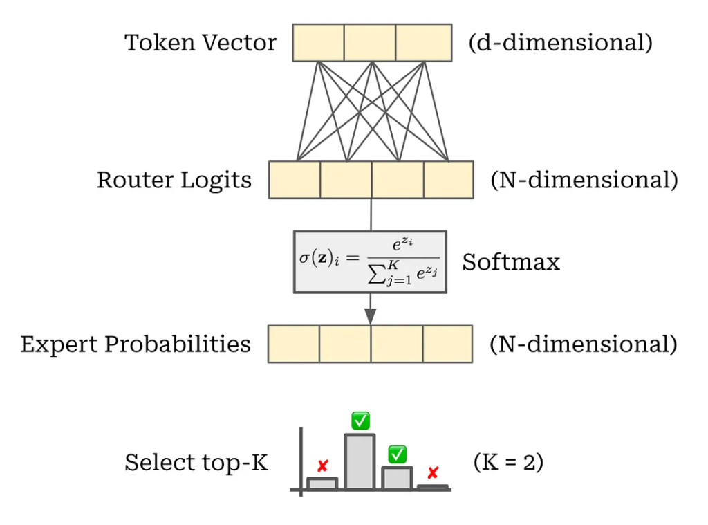
One of the simplest ways to route tokens to experts is to use a linear layer as the router.
Suppose a token is represented by a vector of dimension d, and our MoE layer contains N experts. The router applies a linear transformation to the token representation and produces N scores — one score for each expert.
We then apply softmax to these scores, converting them into a probability distribution across all experts.
For example:
Token vector → Linear layer → N expert scores → Softmax → Expert probabilities
We can then select the top-K experts with the highest probabilities and route the token to those experts.
The top-K probability values are also important because they tell us how strongly the router prefers each selected expert. These probabilities can later be used when combining the outputs from the selected experts.
What Does the Router Return?
For each input token, the router typically produces two things:
- Top-
Kexpert indices — which experts were selected for the token. - Top-
Kexpert probabilities — the routing weights associated with those selected experts.
For example, suppose we have 8 experts and K = 2. The router might determine that:
Expert 3 → 0.72Expert 7 → 0.21
The token would therefore be routed to experts 3 and 7, with their respective probabilities used as routing weights.
Why Is This Approach Useful?
The router itself is surprisingly simple — essentially just a linear layer followed by softmax and top-K selection.
Despite its simplicity, this approach provides an effective way to dynamically decide which experts should process each token. Many modern MoE architectures use variations of this basic linear routing + softmax idea.
The overall process can be summarized as:
Token → Linear Router → Softmax → Top-K Selection → Selected Experts
This simple routing mechanism is the foundation for understanding how tokens are dynamically distributed across experts in an MoE model.
import torch
from torch import nn
from torch.nn import functional as F

class BasicSoftmaxRouter(nn.Module):
    def __init__(
            self,
            d,
            n_exp = 8,
            top_k = 2,
            use_noisy_top_k = True,
        ):
    """
    Arguments:
        d: size of embedding dimension
        n_exp: the number of experts to create in the expert layer
        top_k: the number of active experts for each token
        use_noisy_top_k: whether to add noise when computing expert output
        """

        super().__init__()

        # router settings
        self.top_k = top_k
        assert self.top_k >= 1 and self.top_k <= n_exp
        self.use_noisy_top_k = use_noisy_top_k

        # linear projection for (noisy) softmax routing
        # no bias used, see page 4 eq (4) in https://arxiv.org/abs/1701.06538
        self.w_g = nn.Linear(d, n_exp, bias=False)
        self.w_noise = nn.Linear(d, n_exp, bias=False) if self.use_noisy_top_k else None

        def forward(self, x):
            # eq (4) in https://arxiv.org/abs/1701.06538
            logits = self.w_g(x) # [B, C, d] -> [B, C, n_exp]
            if self.use_noisy_top_k:
                # (optionally) add noise into the router
                noise = F.softplus(self.w_noise(x))
                noise *= torch.randn_like(noise)
                logits += noise
                top_k_logits, top_k_indices = logits.topk(self.top_k, dim=-1) # [B, C, k]
                return top_k_logits, top_k_indices
Adding Noise to the MoE Router
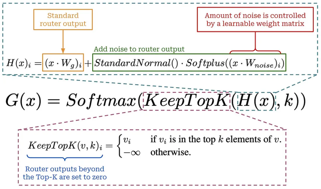
We can also make the routing mechanism slightly more flexible by adding noise to the router’s output.
This idea was introduced in some of the early work on applying Mixture-of-Experts to neural networks. The basic idea is simple: before selecting the top-K experts, we add a small amount of learnable noise to the routing scores.
The process becomes:
Token → Linear Router → Add Noise → Softmax → Top-K Experts
Why add noise?
Without any randomness or variation, the router may repeatedly send tokens to the same experts during training. Adding a small amount of noise can encourage the router to explore different experts and can act as a form of regularization.
This can be particularly useful during training because it may help prevent the routing mechanism from becoming too rigid or overly dependent on a small subset of experts.
The important point is that the noise is not the main routing mechanism. It is an optional addition that can influence the router’s decisions during training.
So, compared with the basic router:
Basic:Linear → Softmax → Top-K
With noisy routing:Linear → Add Learnable Noise → Softmax → Top-K
This small modification can make the training process more robust and encourage better use of the available experts.
Active Parameters
One of the important concepts in an MoE model is active parameters.
Since the router sends each token to only a small subset of the available experts, we don’t use the entire model for every token. Only the parameters belonging to the selected experts are actually involved in processing that token.
For example, suppose an MoE layer has 32 experts, but the router selects only K = 2 experts for each token. The model still contains the parameters of all 32 experts, but only the parameters of those 2 selected experts are active for that particular token.
This gives us an important distinction:
Total parameters → All parameters stored in the model
Active parameters → Parameters actually used for a particular token
As a result, the computational cost of an MoE layer is largely determined by the active parameters, rather than the total number of parameters in the model.
This is what allows MoE models to have a very large parameter count while keeping the amount of computation per token relatively controlled.
Expert Capacity
Sparse routing introduces another practical challenge: how many tokens should each expert be allowed to process?
The router dynamically decides which experts should receive each token. Because these decisions depend on the input, different experts can receive very different numbers of tokens.
For example, in one batch, the router might send:
- Expert 1 → 100 tokens
- Expert 2 → 85 tokens
- Expert 3 → 20 tokens
- Expert 4 → 150 tokens
The number of tokens assigned to each expert can therefore vary from batch to batch.
This creates a problem for efficient hardware execution. GPUs and other accelerators work more efficiently when tensor operations have predictable, fixed shapes.
To address this, MoE implementations typically define an expert capacity — the maximum number of tokens that an expert can process in a given batch.
Conceptually:
Router → Assign tokens to experts → Apply capacity limit → Process tokens
If an expert receives more tokens than its capacity allows, the excess tokens are considered overflow tokens. Depending on the architecture and implementation, these tokens may be handled using mechanisms such as a residual connection or another fallback strategy.
Why Expert Capacity Matters
Expert capacity creates a trade-off:
- Higher capacity → Fewer tokens are dropped or rerouted, but more computation and memory may be required.
- Lower capacity → Better efficiency, but more tokens may exceed the expert’s capacity.
So, while sparse routing makes MoE models computationally efficient, it also introduces an important engineering challenge: efficiently handling a dynamic number of tokens being routed to each expert.
This is where expert capacity, routing strategies, token dispatch, and load balancing become important parts of an MoE implementation.
Expert Capacity
One of the challenges with MoE models is that the router can send different numbers of tokens to different experts. This creates variable-sized inputs, which aren’t ideal for efficient GPU computation.
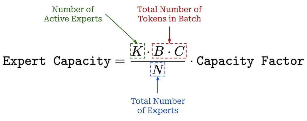
A common solution is to give every expert the same fixed batch size. This fixed limit is called the expert capacity.
In simple terms, expert capacity defines the maximum number of tokens that can be routed to a particular expert within a batch.
For example, if the expert capacity is 64, each expert is allocated space for up to 64 tokens, regardless of how many tokens the router actually sends to it.
This fixed-size approach makes it easier for GPUs and other accelerators to process the expert computations efficiently.
Capacity Factor
The expert capacity is typically controlled using a parameter called the capacity factor.
A capacity factor determines how much capacity is allocated to each expert relative to the expected number of tokens that should be routed there.
A capacity factor of 1.0 provides capacity based on the assumption of relatively balanced routing.
Increasing the capacity factor above 1.0 provides additional room for cases where some experts receive more tokens than others.
For example:
Capacity factor = 1.0
→ Less extra capacity
→ Lower memory usage
→ Higher efficiency
→ Less tolerance for uneven routing
Capacity factor > 1.0
→ More buffer for overloaded experts
→ Lower risk of token overflow
→ Higher memory usage
→ Potentially lower efficiency
So, the capacity factor is essentially a trade-off between efficiency and routing flexibility.
The key idea is:
Router → Assign tokens → Expert capacity limits tokens per expert → Experts process fixed-size batches
Choosing an appropriate capacity is important because it helps balance hardware utilization, memory consumption, and the risk of tokens exceeding an expert’s capacity.
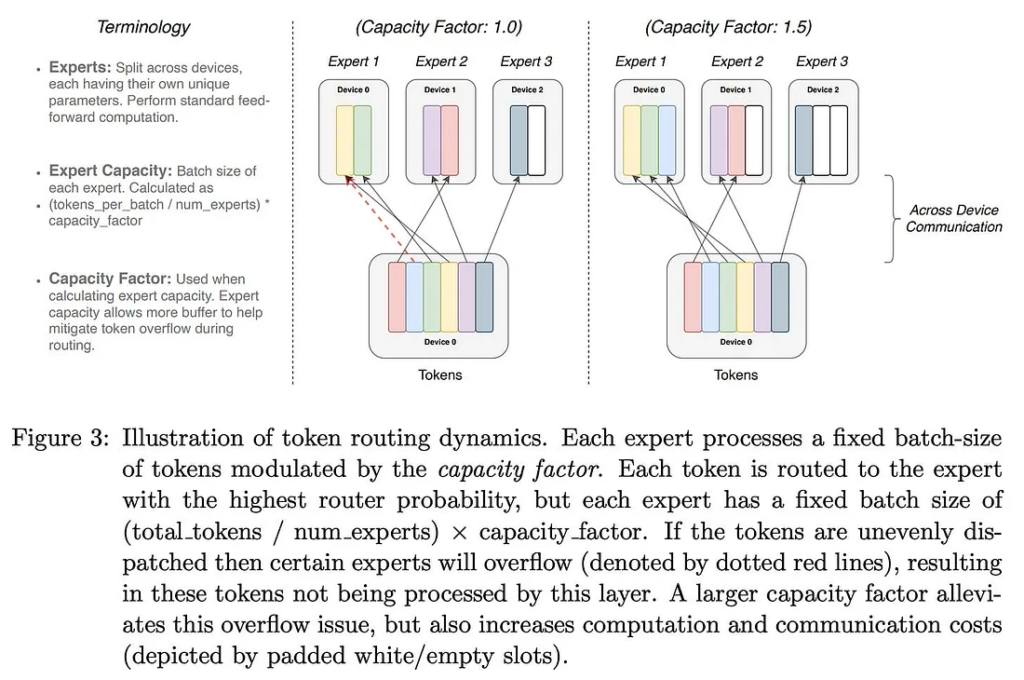
Handling Tokens That Exceed Expert Capacity
If more tokens are routed to an expert than its capacity allows, the extra tokens cannot be processed by that expert. These tokens are therefore dropped from the expert computation.
Importantly, dropping a token does not mean removing it from the model completely. Instead, the token’s current representation is passed forward through the residual connection, allowing it to continue to the next Transformer layer without being processed by that expert.
The goal is to keep the number of dropped tokens as small as possible. MoE models can work effectively with relatively low capacity factors, but if the capacity is set too low, too many tokens may be skipped, which can affect model quality.
The capacity factor does not have to be the same during training and evaluation. For example, the ST-MoE architecture uses a capacity factor of 1.25 during training and 2.0 during evaluation.
PyTorch Implementation
Now that we understand how routing, expert selection, and expert capacity work, we can put everything together and build a fully functional MoE router.
The basic routing mechanism is still the same as before:
Linear Router → Softmax → Top-K Expert Selection
However, the implementation now has an additional responsibility: it needs to create fixed-size input tensors for each expert while respecting the expert capacity.
Because of this, the PyTorch implementation is more involved than the simple router we saw earlier.
The implementation can be broken down into a few main steps:
- Lines 41–47: Compute the output of the noisy linear router.
- Lines 49–52: Select the top-
Kexperts for each token and obtain their corresponding routing probabilities. - Lines 55–58: Calculate the expert capacity, which determines the maximum number of tokens each expert can process.
- Lines 60–88: Use PyTorch indexing and tensor operations to assign tokens to experts while respecting the capacity limit.
- Lines 90–93: Assemble the resulting tensors into the final fixed-size batches of expert inputs.
The code may look complicated because there is a lot of tensor manipulation happening behind the scenes. But conceptually, the router is doing something quite straightforward:
Token representations → Router scores → Top-K experts → Apply capacity limit → Build fixed-size expert batches
Once these batches have been created, the experts can process their assigned tokens efficiently using batched operations.
The important takeaway is that expert capacity turns dynamic token routing into fixed-size computations, making sparse MoE layers much easier to execute efficiently on modern hardware.
import math

import torch
from torch import nn
from torch.nn import functional as F

class Router(nn.Module):
    def __init__(
            self,
            d,
            n_exp = 8,
            top_k = 2,
            use_noisy_top_k = True,
            capacity_factor = 1.25,
        ):
    """
    Arguments:
        d: size of embedding dimension
        n_exp: the number of experts to create in the expert layer
        top_k: the number of active experts for each token
        use_noisy_top_k: whether to add noise when computing expert output
        capacity_factor: used to compute expert capacity
        """

        super().__init__()

        self.d = d
        self.n_exp = n_exp
        self.top_k = top_k
        assert self.top_k >= 1 and self.top_k <= n_exp
        self.use_noisy_top_k = use_noisy_top_k
        self.capacity_factor = capacity_factor
        self.w_g = nn.Linear(d, n_exp, bias=False)
        self.w_noise = nn.Linear(d, n_exp, bias=False) if self.use_noisy_top_k else None

        def forward(self, x):
            # get the total number of tokens in the batch
            B, C, _ = x.size()
            num_tokens = B * C

            # eq (4) in https://arxiv.org/abs/1701.06538
            logits = self.w_g(x) # [B, C, d] -> [B, C, n_exp]
            if self.use_noisy_top_k:
                # (optionally) add noise into the router
                noise = F.softplus(self.w_noise(x))
                noise *= torch.randn_like(noise)
                logits += noise

                # top-K expert selection, compute probabilities over active experts
                top_k_logits, top_k_indices = logits.topk(self.top_k, dim=-1) # [B, C, K]
                router_probs = torch.full_like(logits, float('-inf')) # [B, C, n_exp]
                router_probs.scatter_(-1, top_k_indices, top_k_logits)
                router_probs = F.softmax(router_probs, dim=-1)

                # compute the expert capacity
                exp_capacity = math.floor(self.top_k * self.capacity_factor * num_tokens / self.n_exp)
                exp_capacity += exp_capacity % 2 # make sure expert capacity is an even integer
                exp_capacity = int(exp_capacity)

                # make a multi-hot mask of chosen experts
                # values are 0 if expert not chosen, 1 if expert chosen
                exp_mask = F.one_hot(top_k_indices, num_classes=self.n_exp) # [B, C, K, n_exp]
                exp_mask = exp_mask.view(num_tokens, self.top_k, self.n_exp) # [B * C, K, n_exp]
                exp_mask = exp_mask.permute(1, 0, 2) # [K, B * C, n_exp]

                # compute index for each token in expert batch
                # NOTE: cumsum counts top-1 first, top-2 second, etc.
                # to prioritize top experts when dropping tokens
                exp_rank = exp_mask.reshape(self.top_k * num_tokens, self.n_exp) # [K * B * C, n_exp]
                exp_rank = torch.cumsum(exp_rank, dim=0) - 1 # cumsum of expert selections [K * B * C, n_exp]
                exp_rank = exp_rank.reshape(self.top_k, num_tokens, self.n_exp) # [K, B * C, n_exp]

                # mask entries beyond expert capacity and compute used capacity
                exp_mask *= torch.lt(exp_rank, exp_capacity) # [K, B * C, n_exp]

                # matrix storing token position in batch of corresponding expert
                exp_rank = torch.sum(exp_mask * exp_rank, dim=-1) # [K, B * C]

                # mask probabilities to only include selected experts
                router_probs = router_probs.view(num_tokens, self.n_exp)[None, :] # [1, B * C, n_exp]
                exp_weights = exp_mask * router_probs # [K, B * C, n_exp]

                # position of each token within the capacity of the selected expert
                exp_rank_sc = F.one_hot(exp_rank, num_classes=exp_capacity) # [K, B * C, exp_capacity]

                # weight of selected expert for each token at position the capacity of that expert
                exp_weights = torch.sum(exp_weights.unsqueeze(3) * exp_rank_sc.unsqueeze(2), dim=0) # [B * C, n_exp, exp_capacity]
                exp_mask = exp_weights.bool() # binary mask of selected experts for each token

                # reshape tokens into batches for each expert, return both weights and batches
                # [n_exp, exp_capacity, B * C] * [B * C, d] -> [n_exp, exp_capacity, n_embd]
                x = x.view(num_tokens, self.d)
                exp_batches = exp_mask.permute(1, 2, 0).type_as(x) @ x
                return exp_weights, exp_mask, exp_batches
Load Balancing and Auxiliary Losses
So far, our routing mechanism selects the top-K experts for each token, but it doesn’t explicitly encourage the router to distribute tokens evenly across all experts.
This can create a problem known as routing collapse.
The router may start favoring a small number of experts and repeatedly send most tokens to them. Those experts then receive more training, while the remaining experts receive fewer tokens and less training. Over time, this can reinforce the router’s original preference:
Favored experts → Receive more tokens → Train more → Become more likely to be selected → Receive even more tokens
As a result, some experts can become overloaded while others are barely used.
This is undesirable because one of the main benefits of an MoE model is having multiple experts that can learn different patterns. If the router consistently uses only a few of them, much of the model’s capacity goes unused.
How Do We Prevent Routing Collapse?
A common solution is to introduce an additional load-balancing loss, also called an auxiliary loss.
This loss encourages the router to distribute tokens and routing probability more evenly across the available experts.
The overall training objective then contains two parts:
Total Loss = Language Modeling Loss + Auxiliary Load-Balancing Loss
The main language-modeling loss teaches the model to make accurate predictions, while the auxiliary loss encourages healthier utilization of the experts.
The goal isn’t necessarily to make every expert receive exactly the same number of tokens. Instead, the auxiliary objective encourages the routing system to avoid consistently overloading a small subset of experts.
This creates a more balanced MoE system where the available experts are actually being used.
In short:
Without load balancing:
Tokens → Router → Same few experts → Overloaded experts + underused experts → Routing collapse
With load balancing:
Tokens → Router → More balanced expert utilization → Better use of model capacity
Load balancing is therefore an important part of making sparse MoE architectures work effectively in practice.
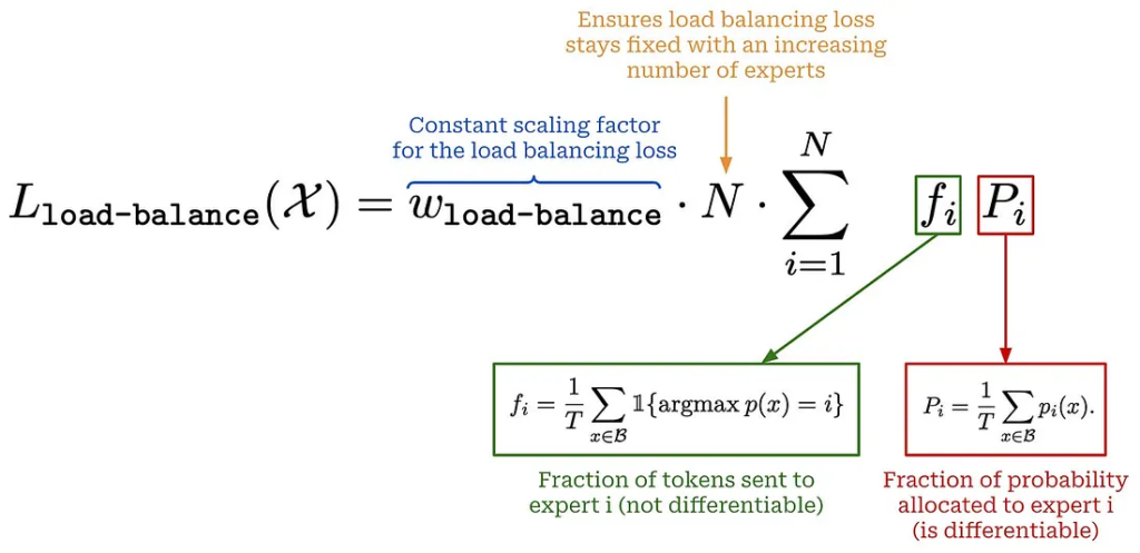
Load Balancing Loss
To prevent routing collapse and encourage the router to make better use of all available experts, we can add an auxiliary load-balancing loss to the training objective.
The idea is straightforward: we want the router to distribute both its routing probabilities and tokens reasonably evenly across the experts.
The load-balancing loss considers two quantities for each expert:
- Fraction of router probability — how much routing probability the router assigns to a particular expert.
- Fraction of tokens dispatched — how many tokens are actually sent to that expert.
If the MoE has N experts, we can represent these two quantities using two N-dimensional vectors:
Probability vector:[p₁, p₂, ..., pₙ]
Token distribution vector:[f₁, f₂, ..., fₙ]
We can then calculate the auxiliary loss using the dot product of these two vectors.
The important intuition is that the loss becomes smaller when the router distributes both probabilities and tokens more uniformly across the experts.
For example, if one expert receives most of the routing probability and most of the tokens, the two distributions become concentrated around that expert, increasing the balancing loss. A more evenly distributed routing pattern produces a lower loss.
The overall training objective can therefore be written conceptually as:
Total Loss = Language Modeling Loss + Load Balancing Loss
The language-modeling loss focuses on prediction quality, while the auxiliary loss encourages the router to make effective use of the available experts.
PyTorch Implementation
The implementation can be broken down into three main steps:
- Lines 9–17: Define the constants and input tensors required to calculate the load-balancing loss.
- Lines 19–24: Calculate the fraction of tokens assigned to each expert.
- Lines 26–27: Calculate the fraction of routing probability assigned to each expert.
- Lines 29–31: Compute a scaled dot product between the token distribution and probability distribution to obtain the final auxiliary loss.
So, conceptually, the calculation is:
Router probabilities → Expert probability distribution
Token assignments → Expert load distribution
Both distributions → Dot product → Auxiliary loss
This additional loss gives the router an incentive to avoid repeatedly selecting the same experts and helps maintain a healthier distribution of work across the MoE layer.
"""
Computes Switch Transformer auxiliary loss (https://arxiv.org/abs/2101.03961)
See equations (4)-(6) on page 7
"""

import torch
import torch.nn.functional as F

# constants
B = 16 # batch size
C = 256 # sequence length
n_exp = 8 # number of experts
K = 2 # number of active expert

# define tensors needed to compute load balancing loss
indices = torch.randint(1, n_exp + 1, (B, C, K)) # top-K indices ([B, C, K])
expert_probs = F.softmax(torch.rand(B, C, n_exp), dim=2) # expert probabilities ([B, C, n_exp])

# equation (5): compute ratio of tokens allocated to each expert
# total number of tokens is defined as total tokens in batch * K
with torch.no_grad():
    one_hot_indices = F.one_hot(indices, num_classes=n_exp) # [B, C, K, n_exp]
    one_hot_indices = torch.sum(one_hot_indices.float(), dim=2) # [B, C, n_exp] (sum over K dimension)
    tokens_per_expert = torch.mean(one_hot_indices.float(), dim=(0, 1))

    # equation (6): compute ratio of router probability allocated to each expert
    prob_per_expert = torch.mean(expert_probs.float(), dim=(0, 1))

    # equation (4): take a scaled dot product between prob / token allocation vectors
    # multiply the result by the number of experts
    load_balance_loss = n_exp * torch.sum(prob_per_expert * tokens_per_expert)
Router Z-Loss
The load-balancing loss helps distribute tokens more evenly across experts, but there is another useful auxiliary loss that can improve the stability of the routing mechanism: the router z-loss.
Unlike the load-balancing loss, which focuses on how tokens and probabilities are distributed across experts, the router z-loss focuses on the size of the router’s logits.
Recall that the router first produces a score for each expert:
Token → Linear Router → Expert Logits → Softmax → Routing Probabilities
The router z-loss is applied to the logits before softmax, not to the resulting probabilities.
The basic idea is to discourage the router from producing extremely large logit values. Keeping these logits under control can make the routing process more numerically stable during training.
So, the two auxiliary losses serve different purposes:
- Load-balancing loss: Encourages tokens and routing probability to be distributed across experts.
- Router z-loss: Encourages the router to keep its pre-softmax logits from becoming excessively large.
Conceptually, the training objective becomes:
Total Loss = Language Modeling Loss + Load Balancing Loss + Router Z-Loss
The router z-loss therefore acts as an additional regularization term for the routing network, helping keep the router’s outputs well-behaved while the model learns which experts to use.
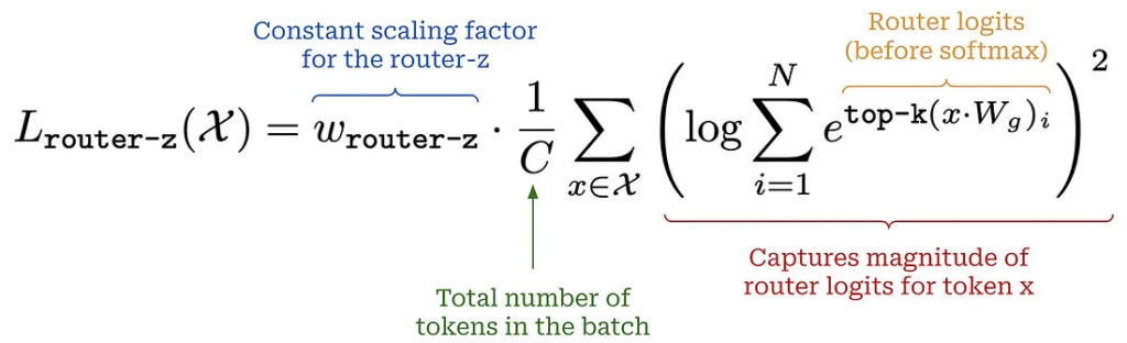
Why Router Z-Loss Is Important
The router produces a score, or logit, for every expert before applying the softmax function. Ideally, these logits should remain within a reasonable range.
The problem is that logits can become extremely large during training. Since softmax involves an exponential operation, large logits can lead to very large intermediate values. This can introduce numerical or round-off errors and, in extreme cases, make training unstable — even when using float32 precision.
The router z-loss addresses this by adding a penalty when the router’s logits become too large. In effect, it encourages the routing network to keep its logits under control.
The idea can be summarized as:
Large router logits → Large exponential values → Numerical instability
Router z-loss → Penalizes large logits → More stable routing
How Is Router Z-Loss Computed?
The implementation can be broken down into three main steps:
- Lines 8–14: Prepare the router logits, which are the raw scores produced by the routing network before softmax is applied.
- Line 21: Compute the logsumexp of the router logits and square the result.
logsumexpis a numerically stable way of performing the equivalent of:log(exp(x₁) + exp(x₂) + … + exp(xₙ))without directly calculating potentially huge exponential values. - Line 24: Average this value across all tokens by summing the results and dividing by the total number of tokens.
Conceptually, the process is:
Router logits → LogSumExp → Square → Average → Router Z-Loss
The resulting value is added to the overall training objective as an auxiliary loss:
Total Loss = Language Modeling Loss + Load Balancing Loss + Router Z-Loss
The two router-related losses address different problems:
- Load-balancing loss → encourages the model to use its experts more evenly.
- Router z-loss → keeps the router’s logits from becoming excessively large and helps improve numerical stability.
Together, they help make the MoE routing mechanism both better balanced and more stable during training.
"""
Computes ST-MoE router z loss (https://arxiv.org/abs/2202.08906)
See equation (5) on page 7
"""

import torch

# constants
B = 16 # batch size
C = 256 # sequence length
n_exp = 8 # number of experts

# create input tensor for router z-loss
router_logits = torch.rand(B, C, n_exp) # [B, C, n_exp]

# exponentiate logits, sum logits of each expert, take log, and square
# code below is equivalent to the following:
    # z_loss = torch.exp(router_logits)
    # z_loss = torch.sum(z_loss, dim=-1)
    # z_loss = torch.log(z_loss) ** 2.0
    router_z_loss = torch.logsumexp(router_logits, dim=-1) ** 2.0 # [B, C]

    # sum over all tokens and divide by total number of tokens
    router_z_loss = torch.mean(router_z_loss)
Combining Auxiliary Losses
Now that we’ve looked at the different auxiliary losses used in MoE models, the natural question is: Do we choose just one of them?
In practice, we can use all of them together.
During training, the standard language modeling loss remains the main objective. We then add the auxiliary losses that help keep the MoE routing system balanced and stable.
Each auxiliary loss is multiplied by its own scaling factor, which controls how strongly it contributes to the overall training objective.
Conceptually:
Total Loss = Language Modeling Loss + α × Load Balancing Loss + β × Router Z-Loss
where:
α= scaling factor for the load-balancing lossβ= scaling factor for the router z-loss
Typical default values are:
- Load-balancing loss:
α = 0.001 - Router z-loss:
β = 0.01
The scaling factors are intentionally small because the language-modeling objective should remain the primary focus of training. The auxiliary losses act more like regularizers, guiding the routing mechanism without overpowering the main learning objective.
So the overall training process looks like:
Language Modeling Loss+
Scaled Load-Balancing Loss+
Scaled Router Z-Loss↓
Total Training Loss
This allows the model to simultaneously learn to predict the next token, distribute tokens across experts, and keep the routing mechanism numerically stable.

Current Research
The auxiliary losses we’ve discussed — particularly the load-balancing loss and router z-loss — can be very useful for making MoE models easier and more stable to train.
However, they also introduce an important trade-off.
The effectiveness of these auxiliary losses depends heavily on their scaling factors. If the weights are set too high, the model may focus too much on balancing and stabilizing the routing process instead of optimizing the main language-modeling objective.
In other words, improving routing stability doesn’t necessarily mean improving the model’s final performance.
A simplified view is:
Too little auxiliary loss → Potentially unstable or poorly balanced routing
Too much auxiliary loss → Better routing stability, but potentially reduced model performance
Finding the right balance is therefore important.
Recent research has continued to explore alternative routing strategies, balancing techniques, and training objectives that can reduce the need for these auxiliary losses while maintaining stable training.
As a result, there is still no single universally optimal recipe for training MoE models. Choosing the right routing mechanism, capacity settings, auxiliary losses, and scaling factors remains an active area of research.
The broader takeaway is that building an MoE architecture is only part of the challenge. Training it effectively is an equally important problem.
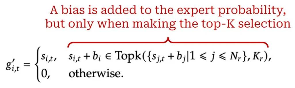
Auxiliary-Loss-Free Load Balancing
A more recent approach to MoE routing is to improve load balancing without relying entirely on an additional load-balancing loss.
For example, DeepSeek-V3 introduced an auxiliary-loss-free load-balancing strategy that adjusts the router’s output using a dynamic bias when selecting the top-K experts.
The basic idea is simple: the system keeps track of how frequently each expert is being selected and adjusts its bias accordingly.
- If an expert is under-utilized, its bias is increased, making it more likely to be selected.
- If an expert is over-utilized, its bias is decreased, making it less likely to be selected.
This creates a feedback loop that encourages a more balanced distribution of tokens across experts.
Conceptually:
Monitor expert usage → Adjust expert biases → Select top-K experts → Monitor usage again → Repeat
For example:
Underused expert → Increase bias → Higher chance of selection
Overused expert → Decrease bias → Lower chance of selection
The amount by which the bias is changed is controlled by a hyperparameter called the bias update speed, typically represented by γ.
After each training step, the system checks the expert load across the batch and adjusts the bias:
Underloaded expert → bias += γ
Overloaded expert → bias -= γ
This approach provides a way to encourage balanced routing directly through the routing mechanism, rather than depending entirely on a large auxiliary loss.
However, auxiliary losses have not necessarily been eliminated completely. DeepSeek-V3 still uses load-balancing losses, but with a smaller scaling factor.
The broader idea is important: instead of forcing balanced routing entirely through the training objective, we can also actively adjust the router based on how experts are being utilized.
This illustrates an ongoing direction in MoE research: finding ways to achieve efficient and balanced expert utilization while minimizing any negative impact on the model’s primary learning objective.
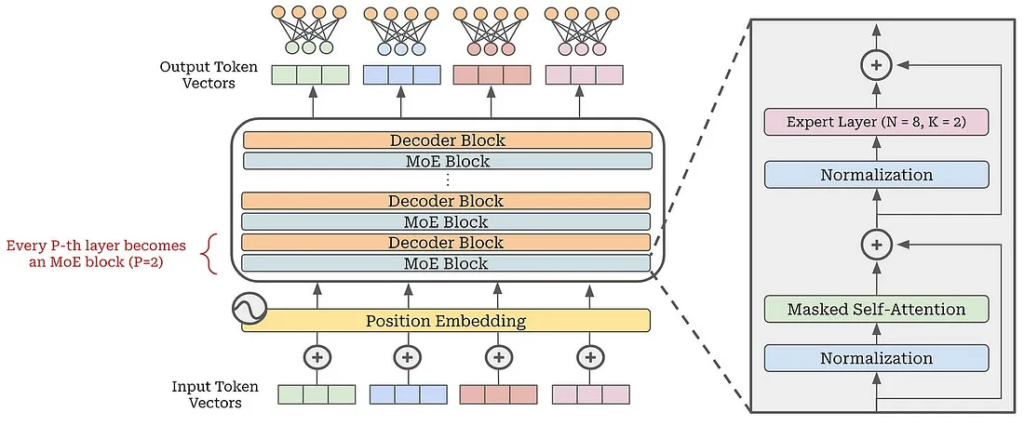
Building the Full MoE Decoder-Only Transformer
At this point, we have covered the main components needed to build an expert layer. Now we can put everything together and create a complete MoE-based decoder-only Transformer.
The overall architecture remains very similar to a standard decoder-only Transformer. The main difference is that some of the feed-forward layers are replaced with MoE expert layers.
An MoE Transformer block contains:
- Masked multi-head self-attention — allows each token to attend to the appropriate previous tokens.
- Expert layer — replaces the standard feed-forward network in selected Transformer blocks.
We don’t necessarily need to use an expert layer in every block. Instead, we can use a stride of P and replace the feed-forward layer with an MoE layer every P-th Transformer block.
For example, with P = 4:
Block 1 → Standard FFN
Block 2 → Standard FFN
Block 3 → Standard FFN
Block 4 → MoE Expert Layer
Block 5 → Standard FFN
Block 6 → Standard FFN
Block 7 → Standard FFN
Block 8 → MoE Expert Layer
This gives us an interleaved MoE architecture.
The rest of the Transformer block remains largely unchanged. We still have the same attention mechanism, normalization, and residual connections.
The key difference can therefore be summarized as:
Standard Transformer:Self-Attention → Feed-Forward Network
MoE Transformer:Self-Attention → Feed-Forward Network
orSelf-Attention → Expert Layer
The expert layer itself contains the additional machinery we’ve discussed:
Router → Top-K Expert Selection → Capacity Handling → Expert Computation → Combine Expert Outputs
Before putting the entire architecture together, we still need to understand one important detail: how the outputs from the selected experts are combined to produce the final output for each token.
Once that final step is defined, we can combine the expert layer with the Transformer blocks to create the complete MoE-based decoder-only Transformer.
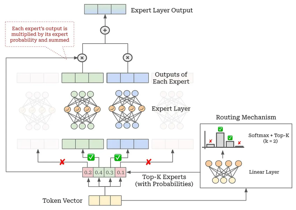
Computing the Output of an MoE Expert Layer
Once the router has determined which experts should process each token, we need to combine their outputs into a single representation for that token.
The process is straightforward:
- Route each token to its selected experts.
- Run the token through those active experts to obtain their individual outputs.
- Combine the expert outputs using the routing probabilities produced by the router.
The routing probabilities act as weights when combining the outputs. An expert with a higher routing probability contributes more to the final representation.
For example, if a token is routed to two experts:
Expert 1 → probability 0.7
Expert 2 → probability 0.3
the final representation is essentially a weighted combination:
Output = 0.7 × Expert₁(token) + 0.3 × Expert₂(token)
This allows the router to control not only which experts process a token, but also how much each expert contributes to the final result.
Shared Experts
Some newer MoE architectures also introduce shared experts.
Unlike routed experts, shared experts are always active for every token. This slightly changes the routing and computation process, but the basic idea remains the same: combine the outputs from the relevant expert computations to produce the final token representation.
PyTorch Implementation
A complete expert-layer implementation brings all these ideas together.
The process can be broken down into three main steps:
- Line 49: The router provides the batches of tokens assigned to each expert, along with the corresponding routing probabilities.
- Line 52: These token batches are passed through their respective feed-forward expert networks to generate the expert outputs.
- Lines 54–58: Each expert output is multiplied by its corresponding routing probability, and the weighted outputs are combined to produce the final output of the MoE layer.
So the complete flow is:
Token representations → Router → Top-K experts → Expert computation → Weight by routing probabilities → Combine → MoE output
The important idea is that the router determines who processes the token, while the routing probabilities determine how much each selected expert contributes to the final representation.
from torch import nn

class MOELayer(nn.Module):
    def __init__(
            self,
            d,
            n_exp = 8,
            top_k = 2,
            use_noisy_top_k = True,
            capacity_factor = 1.25,
            bias=False,
            dropout=0.2,
        ):
    """
    Arguments:
        d: size of embedding dimension
        n_exp: the number of experts to create in the expert layer
        top_k: the number of active experts for each token
        use_noisy_top_k: whether to add noise when computing expert output
        capacity_factor: used to compute expert capacity
        bias: whether or not to use bias in linear layers
        dropout: probability of dropout
        """

        super().__init__()
        self.router = Router( # (noisy) top k router
            d=d,
            n_exp=n_exp,
            top_k=top_k,
            use_noisy_top_k=use_noisy_top_k,
            capacity_factor=capacity_factor,
        )
    self.experts = MLPExperts( # group of MLPs (experts)
        d=d,
        n_exp=n_exp,
        bias=bias,
        dropout=dropout,
    )

def forward(self, x: torch.Tensor):
    B, C, d = x.size() # track original shape of input
    num_tokens = (B * C)

    # pass each token through the router
    exp_weight, exp_mask, exp_batches = self.router(x)

    # compute expert output
    exp_out = self.experts(exp_batches) # [n_exp, exp_capacity, d]

    # aggregate expert outputs based on router weights
    # eq (2) on page 4 of ST-MoE (https://arxiv.org/abs/2202.08906)
    exp_weight = exp_weight.view(num_tokens, -1) # [B * C, n_exp * exp_capacity]
    exp_out = exp_out.view(-1, d) # [n_exp * exp_capacity, d]
    output = exp_weight @ exp_out # [B * C, d]

    # resize output before return
    return output.view(B, T, d)
MoE in PyTorch
Now that we have implemented the expert layer, we can integrate it into our existing decoder-only Transformer block.
The modification is actually quite small. Instead of always using the standard feed-forward MLP module, we make the block capable of using either the regular MLP or our new MoELayer.
In other words, the original Transformer block:
Masked Self-Attention → MLP
can optionally become:
Masked Self-Attention → MoELayer
The MoELayer acts as a drop-in replacement for the original feed-forward network. Internally, it handles the router, expert selection, capacity management, expert computation, and combination of the expert outputs.
This gives us an MoEBlock that retains the overall structure of the standard Transformer block while replacing its feed-forward component with a sparse expert layer when required.
Conceptually:
Standard Block
Input → Attention → MLP → Output
MoE Block
Input → Attention → Router → Selected Experts → Combine Outputs → Output
This design is useful because the rest of the Transformer architecture doesn’t need to change. We can reuse the same attention, normalization, and residual-connection components and simply swap the feed-forward module when we want to introduce MoE functionality.
That makes the MoE architecture a relatively clean extension of the standard decoder-only Transformer.
from torch import nn

class MoEBlock(nn.Module):

    def __init__(
            self,
            d,
            H,
            C,
            n_exp,
            top_k,
            use_noisy_top_k = True,
            capacity_factor = 1.25,
            bias = False,
            dropout = 0.2,
        ):
    """
    Arguments:
        d: size of embedding dimension
        H: number of attention heads
        C: maximum length of input sequences (in tokens)
        n_exp: the number of experts to create in the expert layer
        top_k: the number of active experts for each token
        use_noisy_top_k: whether to add noise when computing expert output
        capacity_factor: used to compute expert capacity
        bias: whether or not to use bias in linear layers
        dropout: probability of dropout
        """

        super().__init__()
        self.ln_1 = nn.LayerNorm(d)
        self.attn = CausalSelfAttention(d, H, T, bias, dropout)
        self.ln_2 = nn.LayerNorm(d)
        self.mlp = MOELayer(
                d,
                n_exp,
                top_k,
                use_noisy_top_k,
                capacity_factor,
                bias,
                dropout,
            )

        def forward(self, x):
            x = x + self.attn(self.ln_1(x))
            x = x + self.mlp(self.ln_2(x))
            return x
Final MoE Architecture
At this point, the final MoE architecture is almost identical to the decoder-only Transformer we built earlier.
The only major change is that we replace every P-th Transformer block with an MoEBlock.
For example, if P = 4, the model would look like:
Block 1 → Standard Transformer Block
Block 2 → Standard Transformer Block
Block 3 → Standard Transformer Block
Block 4 → MoE Block
Block 5 → Standard Transformer Block
Block 6 → Standard Transformer Block
Block 7 → Standard Transformer Block
Block 8 → MoE Block
…
Everything else — token embeddings, positional embeddings, attention, normalization, residual connections, and the final output layer — remains essentially the same as in the standard GPT implementation.
So the overall idea is simple:
GPT architecture + interleaved MoE blocks = MoE-based GPT
Pretraining nanoMoE from Scratch
Now that we understand how the individual MoE components work, we can put everything together and pretrain an LLM from scratch using this architecture.
The implementation described here is called nanoMoE and is based on Andrej Karpathy’s nanoGPT project. The main difference is that the standard GPT architecture has been modified to support an MoE-based decoder-only Transformer.
The nanoMoE implementation brings together the routing, expert layers, capacity management, load balancing, and other MoE components we’ve discussed throughout this section.
The project is organized around a few key components:
- Model implementation: The
GPTmodel definition has been extended to support MoE blocks alongside the standard Transformer blocks. - Training: The training code remains largely based on the original nanoGPT training implementation.
- Dataset: nanoMoE is pretrained on a 25-billion-token subset of OpenWebText.
- Configuration: The training configuration defines the architecture and hyperparameters used for the nanoMoE pretraining run.
The important takeaway is that we don’t need to redesign the entire GPT architecture to introduce MoE. Instead, we can build the expert machinery and then integrate it into selected Transformer blocks.
Best Practices for Training MoEs
Although MoE architectures are conceptually similar to standard Transformer models, they are generally more complicated to train.
There are several reasons for this, including:
- Dynamic routing of tokens between experts
- Expert capacity constraints
- Load balancing
- Communication between devices
- Router instability
- Additional auxiliary losses
- Uneven utilization of experts
This raises an important question:
If an MoE model only makes relatively small architectural changes to a standard Transformer, why can it be more difficult to train?
The answer lies primarily in the routing mechanism.
In a dense Transformer, every token follows essentially the same computational path through each layer. In an MoE model, however, the path depends on the router’s decisions.
A small change in routing can therefore change:
- Which experts receive tokens
- How many tokens each expert processes
- Which experts receive more gradient updates
- Whether some experts become overloaded
- How effectively the model uses its total parameter capacity
This creates a feedback loop between routing and learning that doesn’t exist to the same extent in a dense Transformer.
As a result, successful MoE pretraining requires careful choices around routing, expert capacity, load balancing, auxiliary losses, initialization, and training hyperparameters.
Understanding these training considerations is the next important step toward successfully pretraining an MoE language model from scratch.
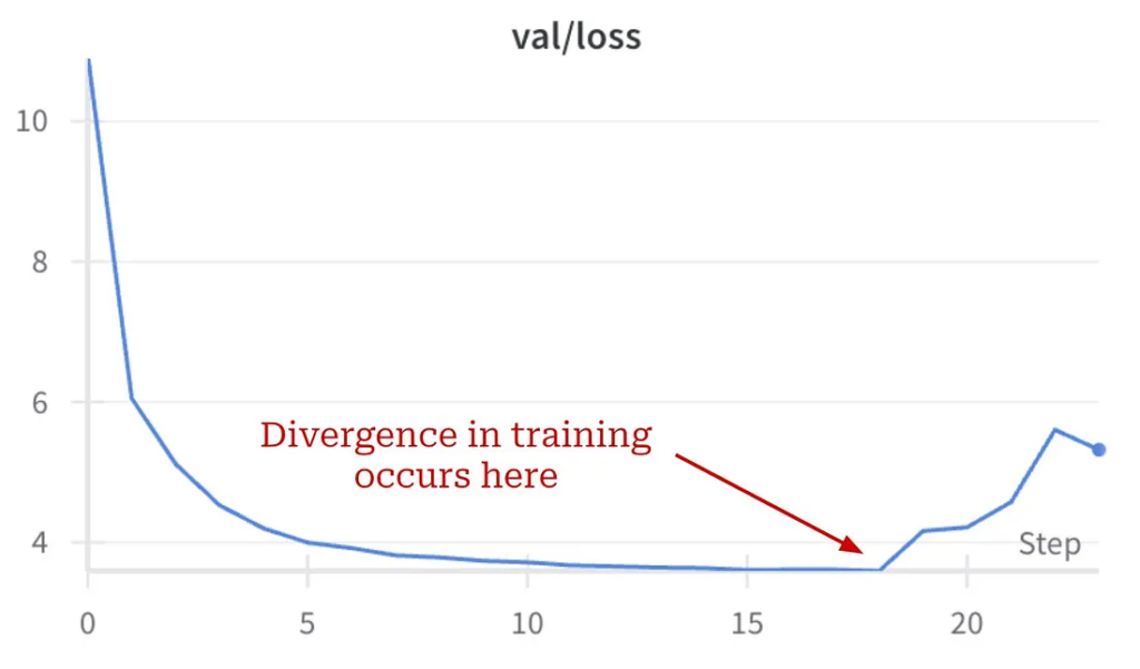
Best Practices for Stable MoE Training
When training an MoE model, two major problems can cause instability:
- Routing collapse — the router starts selecting the same few experts repeatedly, leaving other experts underused.
- Numerical instability — the router can produce very large values, particularly because softmax involves exponential operations. This can lead to round-off errors and eventually destabilize training.
When either problem becomes severe, the training loss can diverge. At that point, training may need to be stopped and restarted from a checkpoint, which wastes both time and GPU resources.
Fortunately, several techniques can make MoE training much more stable.
1. Use Auxiliary Losses
As discussed earlier, we don’t need to choose between the different auxiliary losses. We can combine them with the standard language-modeling loss.
For nanoMoE, we use both:
- Load-balancing loss — encourages tokens to be distributed more evenly across experts.
- Router z-loss — keeps router logits under control and improves numerical stability.
Together, these losses help prevent routing collapse and encourage more consistent expert utilization.
2. Use Mixed Precision Carefully
Mixed-precision training is widely used when training LLMs because it can significantly reduce memory usage and computation compared with running the entire model in float32.
PyTorch provides Automatic Mixed Precision (AMP), which makes this relatively easy to enable.
Common lower-precision formats include:
float16bfloat16FP8in some newer large-scale training systems
However, the MoE router needs special treatment.
Because the router relies on softmax and exponential operations, performing its calculations in lower precision can increase numerical errors. Even when the rest of the model uses mixed precision, it is therefore useful to keep the router computation in full float32 precision.
Conceptually:
Most model → Mixed precision
MoE router → float32
In PyTorch, AMP can be disabled around the router computation:
with torch.amp.autocast(device_type="cuda", enabled=False):
    # Router computation runs in float32
    ...
This small exception can improve routing stability without giving up the efficiency benefits of mixed-precision training for the rest of the model.
3. Use an Appropriate Weight Initialization
Weight initialization has always been important for training deep neural networks. Techniques such as Glorot/Xavier and He initialization helped make it possible to train increasingly deep networks reliably.
MoE models can benefit from similar ideas, but some work has proposed modified initialization schemes specifically for MoE training.
One approach initializes weights using a truncated normal distribution with:
σ = √(s / n)
where:
s= scale hyperparametern= fan-in, or the number of input features to the layer
The weights are centered around zero and truncated to remain within a reasonable range.
A reduced scale such as:
s = 0.1
can also be used to reduce the likelihood of unstable training.
The main idea is simple:
Careful initialization → Better-controlled activations → More stable MoE training
4. Be Careful When Fine-Tuning MoEs
Although this section focuses mainly on pretraining, fine-tuning an MoE model introduces another challenge: overfitting.
MoE models can contain a very large number of parameters, which is useful when training on massive datasets but can become problematic when fine-tuning on a relatively small dataset.
A large model can quickly memorize a small fine-tuning dataset.
Therefore, when fine-tuning an MoE model, techniques such as stronger regularization or a higher dropout rate may be worth considering.
nanoMoE Pretraining Experiments
Now that we understand the techniques that can improve MoE stability, we can test them by pretraining nanoMoE from scratch.
The experiments described here were designed to run on relatively modest hardware: two NVIDIA RTX 3090 GPUs, each with 24 GB of memory.
Because of the hardware constraints, the model and training setup were scaled down so that the complete experiment could fit within GPU memory and finish in roughly a few days.
General Pretraining Configuration
The nanoMoE configuration uses:
| Setting | Value |
|---|---|
| Transformer layers | 6 |
| Attention heads | 6 |
Model dimension d | 368 |
Total experts N | 8 |
Active experts K | 2 |
MoE frequency P | 2 |
| Training capacity factor | 1.25 |
| Evaluation capacity factor | 2.0 |
| Precision | bfloat16 |
| Router precision | float32 |
The model uses an interleaved MoE architecture, meaning every other Transformer block contains an MoE layer.
Learning Rate
The learning-rate schedule follows a common LLM training pattern.
Training begins with a linear warmup, increasing the learning rate from:
6 × 10⁻⁵ → 6 × 10⁻⁴
After reaching the peak learning rate, training switches to cosine decay, eventually reducing the learning rate back toward:
6 × 10⁻⁵
The model also uses the modified weight-initialization strategy described earlier.
Pretraining Dataset
nanoMoE uses the OpenWebText dataset, similar to nanoGPT.
For this experiment, training is performed on approximately 25 billion tokens, which is a smaller-scale setup designed to fit the available hardware.
With the two RTX 3090 GPUs used for the experiment, this setup can complete in roughly five days.
A larger-scale run could use substantially more powerful hardware and a larger number of training iterations.
Stability Experiments
To understand which techniques actually help, five training configurations are compared.
The experiments start with a baseline model that does not use the recommended stability techniques. The improvements are then introduced incrementally:
- Baseline MoE
- Add load-balancing loss
- Add router z-loss
- Run the router in full
float32precision - Use the improved weight-initialization scheme
The baseline configuration suffers from poor expert utilization and eventually becomes unstable.
As the individual improvements are introduced, training becomes progressively more stable. The divergence point is pushed further into training with each improvement.
Most importantly, when all of the techniques are enabled together, nanoMoE is able to complete the entire training run without the instability observed in the baseline experiment.
This provides a useful practical lesson: MoE training stability usually doesn’t come from a single trick. It comes from combining several carefully chosen techniques — balanced routing, stable router computation, appropriate precision, and suitable initialization.
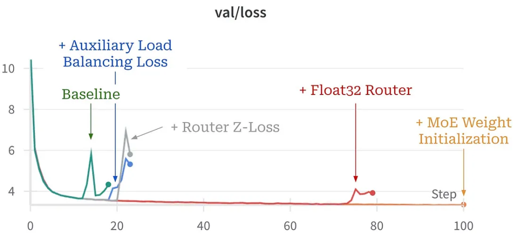
Running nanoMoE Yourself
If you want to experiment with MoE models yourself, nanoMoE provides a useful starting point.
You can modify the training configuration and launch the pretraining process using torchrun. The following command assumes that you’re running the training on a single node with one or more GPUs:
torchrun --standalone --nproc_per_node=<number of GPUs> train.py <path to config>
For example:
torchrun --standalone --nproc_per_node=2 train.py config/train_nano_moe.py
Here, --nproc_per_node specifies how many GPUs should participate in the training process, while the configuration file defines the model architecture and training hyperparameters.
This makes it relatively easy to experiment with different MoE settings, such as:
- Number of experts
- Number of active experts
- Expert capacity
- MoE layer frequency
- Auxiliary-loss scaling factors
- Learning rate
- Precision
- Model size
Further Learning: Mixture-of-Experts
At this point, we’ve covered the major ideas behind Mixture-of-Experts (MoE) language models.
We started with a standard decoder-only Transformer and gradually modified it to create an MoE architecture:
Decoder-only Transformer
→ Replace selected FFN layers with expert layers
→ Add a router
→ Select top-K experts
→ Handle expert capacity
→ Combine expert outputs
→ Add load-balancing mechanisms
→ Stabilize router computation
→ Train the complete MoE model
We then applied these ideas by pretraining a mid-sized MoE language model, nanoMoE, from scratch on the OpenWebText dataset.
The experiments demonstrate that although MoE models introduce additional training challenges, techniques such as auxiliary losses, mixed precision with a full-precision router, careful weight initialization, and expert load balancing can make training much more stable.
Moving Beyond nanoMoE
nanoMoE is primarily a learning and experimentation tool. Real-world MoE systems are considerably more sophisticated.
Production-scale implementations need to deal with additional challenges such as:
- Distributed expert computation
- Communication between GPUs and nodes
- Efficient token dispatch
- Expert parallelism
- Memory optimization
- Large-scale inference
- Dynamic routing at high throughput
- Expert load balancing across hardware
To explore these topics further, it’s useful to study production-oriented MoE frameworks and recent research systems such as OpenMoE, MegaBlocks, Mixtral, DeepSeek-V3, and DBRX.
These systems provide a bridge between the relatively simple nanoMoE implementation and the much more complex MoE architectures used in modern LLM research.
The key takeaway is that the fundamental ideas remain the same:
Route tokens → Activate a small subset of experts → Process tokens sparsely → Combine expert outputs
What changes at larger scales is the engineering required to make this process fast, balanced, memory-efficient, and stable across many GPUs.
Conclusion
MoE is powerful because it separates model capacity from per-token compute. By routing each token to a small number of experts, an MoE LLM can hold many more parameters than a dense model while keeping inference and training more efficient than activating every layer for every token.
The nanoMoE implementation shows the practical side of this idea: a standard decoder-only Transformer can become an MoE model by replacing selected feed-forward layers with routed expert layers. The hard parts are not only writing the PyTorch modules, but also making routing stable, balancing expert usage, handling capacity limits, and choosing auxiliary losses carefully.
FAQs
Primary MoE References
For deeper MoE study, see the ST-MoE research paper, the DeepSeek-V2 technical report, the DeepSeek-V3 technical report, the official PyTorch documentation, and GenAITrail’s internal GLM-5.3 explained guide.
