Multi-Head Latent Attention (MLA): How DeepSeek Reduces the KV Cache

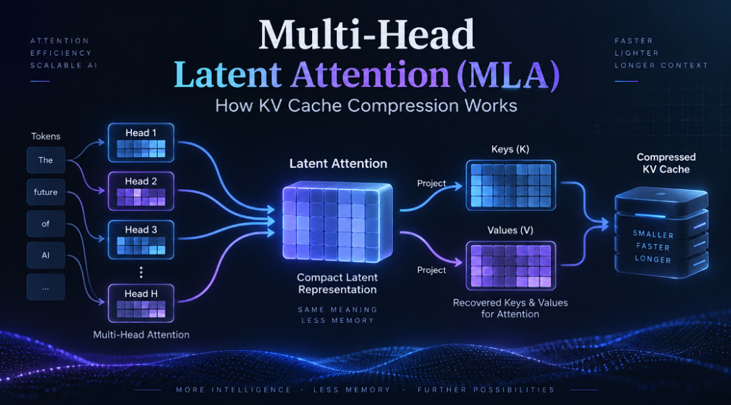
Run a transformer with a short prompt and the attention mechanism may not look particularly problematic. Increase the context to tens of thousands of tokens, serve several users simultaneously, and generate tokens autoregressively, however, and a different bottleneck appears: the KV cache.

Traditional Multi-Head Attention stores a key vector and a value vector for every previous token, for every attention head, in every transformer layer. As context length and batch size increase, those stored tensors can consume several gigabytes of GPU memory.

Multi-Head Latent Attention (MLA) approaches this problem differently.

Instead of storing the complete key and value representations for every attention head, MLA compresses information into a much smaller latent representation. During inference, the model can work from this compressed representation rather than maintaining the full conventional KV cache.

MLA was introduced with DeepSeek-V2. DeepSeek described it as a low-rank joint compression mechanism for keys and values and reported a 93.3% KV-cache reduction for DeepSeek-V2 compared with DeepSeek 67B, alongside substantially higher maximum generation throughput. Those figures are specific to that model comparison rather than a universal property of every MLA architecture.

The architecture was subsequently retained in DeepSeek-V3, whose technical report identifies Multi-Head Latent Attention as one of the model’s core architectural components.

The most interesting part of MLA is not simply that it compresses tensors. The clever part is what gets compressed, what remains uncompressed, and how the projection matrices can be reorganized during inference.

That is where MLA differs from simply reducing the number of KV heads.

Why DeepSeek matters for MLA

DeepSeek matters in this article because DeepSeek made Multi-Head Latent Attention visible to many engineers who were comparing long-context inference costs. DeepSeek-V2 introduced the MLA design, and DeepSeek-V3 kept the same family of ideas because DeepSeek needed lower KV-cache pressure at scale.

When people search for DeepSeek architecture, they usually want more than a high-level diagram. They want to know how DeepSeek reduces memory, how DeepSeek handles RoPE, and why DeepSeek can serve long contexts more efficiently than a plain attention baseline.

This guide therefore treats DeepSeek as the practical case study. The math explains the architecture, the code shows the simplified mechanism, and the DeepSeek source links show where the production implementation differs from the educational version.

That distinction is important: DeepSeek is not just a model name here. DeepSeek is the reference point for understanding why MLA, compressed KV cache design, and optimized inference kernels became a serious topic for LLM deployment.

What problem does Multi-Head Latent Attention solve?

To understand MLA, first consider ordinary Multi-Head Attention.

Given the hidden state of token $t$ , $h_t \in \mathbb{R}^{d}$

the transformer computes query, key, and value representations: $q_t = W^Q h_t$ $k_t = W^K h_t$ $v_t = W^V h_t$

These vectors are divided across multiple attention heads.

For a model with $n_h$ attention heads and a head dimension of $d_h$ , the key and value representations contain roughly: $n_h d_h$

elements each.

During autoregressive generation, queries are required only for the token currently being processed. Previous keys and values are different: the model repeatedly needs them when each new token attends to the existing sequence.

Recomputing every previous key and value at every generation step would be wasteful, so inference engines keep them in a KV cache.

For standard MHA, the storage requirement per token per layer is approximately: $2n_h d_h$

scalar values.

The factor of two comes from storing both K and V.

DeepSeek explicitly identifies this large KV cache as an inference bottleneck for conventional Multi-Head Attention.

This becomes increasingly important as context length grows.

Suppose an illustrative transformer uses:

32 attention heads
128 dimensions per head
BF16 values requiring 2 bytes each

Standard MHA stores: $2 \times 32 \times 128 = 8192$

values per token per layer.

In BF16: $8192 \times 2 = 16,384\text{ bytes}$

That is 16 KB for one token in one layer.

Now multiply that by thousands of tokens, dozens of layers, and several simultaneous requests.

The cache quickly becomes expensive.

How Multi-Head Latent Attention works

The key idea behind MLA is surprisingly simple:

Do not cache the large expanded keys and values if they can be reconstructed from something much smaller.

Instead, MLA takes the hidden state and performs a down-projection: $c_t^{KV} = W^{DKV}h_t$

where $c_t^{KV}$ is a lower-dimensional latent representation.

The model can then generate content keys and values through up-projections: $k_t^C = W^{UK}c_t^{KV}$ $v_t^C = W^{UV}c_t^{KV}$

The important dimensional relationship is: $d_c \ll n_h d_h$

where $d_c$ is the dimension of the compressed KV latent.

Instead of storing all expanded per-head keys and values, the model can primarily cache: $c_t^{KV}$

DeepSeek’s original MLA formulation describes exactly this low-rank joint KV compression.

Conceptually, the data flow changes from:

Standard Multi-Head Attention

hidden state
     │
     ├────────► Key projections ─────► cache K
     │
     └────────► Value projections ───► cache V

to:

Multi-Head Latent Attention

hidden state
     │
     ▼
KV down-projection
     │
     ▼
compressed latent cKV ───────────────► cache
     │
     ├────────► K up-projection
     │
     └────────► V up-projection

That compressed bottleneck is the foundation of MLA.

Why is it called “latent” attention?

The word latent refers to the compressed internal representation used between the original hidden state and the expanded key/value representations.

Rather than treating K and V as the state that must be retained directly, MLA stores an intermediate representation from which their useful information can be obtained.

A useful analogy is storing a compressed source file rather than multiple expanded copies.

The analogy is imperfect because the compression is learned rather than using something like ZIP compression, but it captures the key idea: the network learns a compact representation that contains information useful for both keys and values.

This is also why MLA should not be confused with merely using smaller head dimensions.

The model learns explicit down-projection and up-projection matrices as part of the architecture.

MLA vs MHA vs GQA vs MQA

MLA is not the first attempt to reduce KV-cache size.

Multi-Query Attention and Grouped-Query Attention were developed for similar reasons.

Attention type	Key/value organization	KV-cache strategy	Main idea
MHA	Separate K/V for every head	Largest	Maximum per-head independence
GQA	Groups of query heads share K/V heads	Smaller than MHA	Reduce number of KV heads
MQA	All query heads share one K/V head	Very small	Maximum KV-head sharing
MLA	Head information derives from a compressed latent	Compressed	Low-rank joint KV representation

With Grouped-Query Attention, several query heads share the same key/value head.

With Multi-Query Attention, all query heads share a single key/value head.

MLA takes another route. Rather than directly sharing a small number of complete K/V heads, it learns a compressed latent representation that can support the attention computation.

DeepSeek’s V2 paper reports that its MLA configuration achieved better model results than the MHA, GQA, and MQA alternatives tested in its architecture while requiring substantially less KV-cache storage than standard MHA. That result should be interpreted as DeepSeek’s model-specific ablation result, not as proof that MLA will outperform every other attention architecture in every model.

A practical MLA KV-cache calculation

The easiest way to understand MLA’s advantage is to calculate it.

Consider this illustrative configuration:

Attention heads:           32
Head dimension:            128
Compressed KV dimension:   512
RoPE key dimension:         64
Precision:                 BF16
Transformer layers:         32
Context length:         128,000

These numbers are an educational example, not a claim that they describe a particular DeepSeek checkpoint.

For standard MHA, the number of cached scalars per token per layer would be: $2 \times 32 \times 128 = 8192$

For MLA, using a compressed latent plus a 64-dimensional positional component: $512 + 64 = 576$

The relative cache size becomes: $\frac{576}{8192}=0.0703$

or roughly 7.0% of the original MHA cache.

The theoretical reduction is therefore approximately: $100\%-7.0\%=93.0\%$

Now convert it into memory.

With BF16, MHA requires: $8192\times2=16,384$

bytes per token per layer.

Across 128,000 tokens and 32 layers: $16,384\times128,000\times32$

which is about 62.5 GiB.

The simplified MLA cache would require: $576\times2\times128,000\times32$

or about 4.39 GiB.

Real inference memory will not exactly equal these figures because implementations also have tensor metadata, allocator behavior, batching, temporary buffers, kernel workspaces, quantization choices, paged-cache layouts and other memory consumers.

But the example demonstrates why KV compression becomes so valuable at long context lengths.

Why doesn’t MLA simply compress K and V and stop there?

This is where the architecture becomes more interesting.

If MLA simply down-projected and then reconstructed K and V every time, it would save cache memory but introduce extra computation.

DeepSeek makes the method more efficient using a technique commonly described as weight absorption.

Consider the content key: $k_t^C = W^{UK}c_t^{KV}$

During attention, a query interacts with that key through a dot product.

Instead of always explicitly producing the expanded key first, the linear transformations can be algebraically reorganized so that the key up-projection is absorbed into the query-side calculation.

Similarly, the value up-projection can be combined with the output projection.

DeepSeek’s MLA description notes that $W^{UK}$ can be absorbed into the query projection and $W^{UV}$ into the output projection during inference, avoiding the need to explicitly reconstruct conventional K and V representations in the optimized path.

This matters because reducing storage without controlling reconstruction cost would solve only part of the problem.

The RoPE problem

There is one complication.

Modern transformers commonly use Rotary Position Embeddings, or RoPE, to encode positional information.

RoPE applies a position-dependent transformation to queries and keys.

That creates a problem for the clean matrix absorption described above.

Suppose an up-projection matrix creates the key and then RoPE transforms it:

latent
  │
  ▼
key up-projection
  │
  ▼
RoPE(position)
  │
  ▼
key

Because the RoPE transformation depends on token position, you cannot generally move the fixed projection matrix across that position-dependent operation and expect the result to stay equivalent.

DeepSeek explains that applying RoPE directly to the compressed content-key path would prevent the key up-projection from being cleanly absorbed into the query-side calculation.

Its solution is decoupled RoPE.

Decoupled RoPE in Multi-Head Latent Attention

MLA separates query/key information into two conceptual parts:

Content component
+
Positional RoPE component

The content component participates in the low-rank compression scheme.

A much smaller, separate component carries the rotary positional information.

Conceptually: $q_{t,i}=[q^C_{t,i};q^R_{t,i}]$

and: $k_{t,i}=[k^C_{t,i};k^R_t]$

where:

$C$ represents content information
$R$ represents the RoPE positional component
$i$ represents an attention head

The positional key component can be shared rather than storing a separate copy for every attention head.

Consequently, the practical MLA cache is not literally only the compressed latent.

It generally includes: $c_t^{KV} + k_t^R$

So the per-token per-layer cache requirement is approximately: $d_c+d_h^R$

rather than: $2n_hd_h$

for conventional MHA.

This detail is frequently lost in simplified explanations of MLA.

Saying that MLA “only stores one latent vector” is directionally useful, but incomplete if the implementation uses the decoupled positional branch.

Query compression in MLA

Keys and values are not the only projections MLA can compress.

The original formulation also defines a compressed query representation: $c_t^Q=W^{DQ}h_t$

followed by: $q_t^C=W^{UQ}c_t^Q$

Unlike KV compression, query compression does not directly reduce the persistent autoregressive KV cache because previous queries do not need to be stored.

Its purpose is more related to reducing projection cost and activation memory during model operation.

An important implementation detail is that query compression is configurable rather than something you should assume every MLA implementation uses identically.

For example, DeepSeek’s published V3 inference code contains both paths: when q_lora_rank is zero it performs a direct query projection; otherwise it uses a query down-projection, normalization and up-projection.

That is an important distinction when reading MLA implementations on GitHub: two pieces of code can both implement MLA correctly while having visibly different query branches.

What DeepSeek’s MLA implementation actually caches

Theory becomes clearer when you look at the DeepSeek inference code, because the DeepSeek implementation shows how the cache is actually represented.

The optimized DeepSeek implementation contains buffers for a compressed KV cache and a separate positional-embedding cache:

self.kv_cache
self.pe_cache

The model computes the compressed KV representation, stores it in kv_cache, and stores the positional key representation separately in pe_cache. The query’s non-positional component is transformed so that attention scores can be calculated directly against the compressed latent.

This matches the theory:

Current token
     │
     ├────► query content ──► transformed query
     │
     └────► query RoPE
                        │
                        ▼
          ┌─────────────────────────┐
Cache ───►│ compressed KV + RoPE K │
          └─────────────────────────┘
                        │
                        ▼
                  attention scores

That optimized path is more representative of production MLA than a tutorial implementation that simply decompresses full K and V on every step.

Code attribution and source notes

The PyTorch examples and Colab experiment in this DeepSeek article are original educational examples written for GenAITrail. They are not copied from DeepSeek’s production repositories and they intentionally simplify production details such as decoupled RoPE, absorbed projections, paged KV cache layouts and FlashMLA kernels.

Architecture claims and implementation comparisons are attributed to the primary sources: the DeepSeek-V2 paper, the DeepSeek-V3 technical report, the DeepSeek-V3 GitHub repository and the FlashMLA GitHub repository.

Short DeepSeek identifier examples such as kv_lora_rank, q_lora_rank, self.kv_cache and self.pe_cache are referenced only to explain the public DeepSeek implementation structure; the full runnable code blocks shown here are original tutorial code.

Multi-Head Latent Attention PyTorch implementation

The following code demonstrates the core compression idea in a deliberately small PyTorch module.

It is educational code rather than a replacement for DeepSeek’s production implementation. To keep the mechanism readable, it does not implement decoupled RoPE, paged KV caching, tensor parallelism, FlashMLA kernels, mixed-precision optimizations or weight absorption.

import math

import torch
import torch.nn as nn
import torch.nn.functional as F


class SimpleMLA(nn.Module):
    """
    Educational Multi-Head Latent Attention.

    Demonstrates:
      - low-rank query projection
      - joint KV latent compression
      - per-head K/V reconstruction

    Omits:
      - decoupled RoPE
      - absorbed inference
      - paged KV cache
      - tensor parallelism
      - fused CUDA kernels
    """

    def __init__(
        self,
        d_model: int = 512,
        n_heads: int = 8,
        q_rank: int = 96,
        kv_rank: int = 64,
    ):
        super().__init__()

        assert d_model % n_heads == 0

        self.d_model = d_model
        self.n_heads = n_heads
        self.head_dim = d_model // n_heads
        self.kv_rank = kv_rank

        # Query low-rank projection
        self.q_down = nn.Linear(d_model, q_rank, bias=False)
        self.q_up = nn.Linear(q_rank, d_model, bias=False)

        # Shared compressed KV latent
        self.kv_down = nn.Linear(d_model, kv_rank, bias=False)

        # Recover head-specific K and V
        self.k_up = nn.Linear(kv_rank, d_model, bias=False)
        self.v_up = nn.Linear(kv_rank, d_model, bias=False)

        self.out_proj = nn.Linear(d_model, d_model, bias=False)

    def split_heads(self, x):
        batch, seq_len, _ = x.shape

        x = x.view(
            batch,
            seq_len,
            self.n_heads,
            self.head_dim,
        )

        return x.transpose(1, 2)

    def merge_heads(self, x):
        batch, heads, seq_len, head_dim = x.shape

        x = x.transpose(1, 2).contiguous()

        return x.view(batch, seq_len, heads * head_dim)

    def forward(self, x):
        # x: [batch, sequence, d_model]

        # Low-rank query path
        q_latent = self.q_down(x)
        q = self.q_up(q_latent)

        # Joint KV compression
        kv_latent = self.kv_down(x)

        # For this simple demonstration we expand K/V again.
        # A production MLA inference path can avoid explicitly
        # materializing them through weight absorption.
        k = self.k_up(kv_latent)
        v = self.v_up(kv_latent)

        q = self.split_heads(q)
        k = self.split_heads(k)
        v = self.split_heads(v)

        scores = torch.matmul(
            q,
            k.transpose(-2, -1)
        ) / math.sqrt(self.head_dim)

        attention = F.softmax(scores, dim=-1)

        output = torch.matmul(attention, v)

        output = self.merge_heads(output)

        return self.out_proj(output)


if __name__ == "__main__":
    torch.manual_seed(42)

    model = SimpleMLA(
        d_model=512,
        n_heads=8,
        q_rank=96,
        kv_rank=64,
    )

    x = torch.randn(2, 128, 512)

    y = model(x)

    print("Input shape :", x.shape)
    print("Output shape:", y.shape)

Run it and you should get:

Input shape : torch.Size([2, 128, 512])
Output shape: torch.Size([2, 128, 512])

The important line is not the final attention multiplication.

It is:

kv_latent = self.kv_down(x)

That tensor is the representation an MLA-style inference system wants to retain rather than storing fully expanded K and V tensors for every attention head.

Why this simple implementation is not production MLA

A common mistake in articles about MLA is showing 30 lines of PyTorch and implying that the code reproduces DeepSeek’s actual attention implementation.

It does not.

A production MLA layer needs to consider at least four additional issues.

First is decoupled RoPE. The positional query and key components have to be treated separately from the compressible content representation.

Second is weight absorption. Simply decompressing the latent into complete K and V tensors during every decoding step leaves performance on the table.

Third is KV-cache management. Real serving systems need efficient cache layouts, batching, variable sequence lengths and frequently paged memory.

Fourth is specialized GPU kernels. Saving memory at the architectural level does not automatically guarantee that GPU execution is efficient.

DeepSeek’s own V3 inference code demonstrates separate naive and optimized MLA paths. In the optimized path, it stores compressed KV and positional caches rather than conventional expanded per-head K/V tensors.

For production-oriented kernels, DeepSeek also maintains FlashMLA, a dedicated project for optimized Multi-Head Latent Attention kernels.

MLA and FlashMLA are not the same thing

These two names are sometimes used interchangeably, but they refer to different layers of the stack.

MLA is the attention architecture.

It describes ideas such as:

low-rank KV compression
decoupled RoPE
compressed inference state
weight absorption

FlashMLA is an optimized implementation/kernel project for executing MLA efficiently on GPUs.

The relationship is similar to the difference between an algorithm and an optimized kernel implementing that algorithm.

You can understand MLA without FlashMLA.

You can also write MLA in plain PyTorch.

But production inference requires much more consideration than getting mathematically correct output from a simple PyTorch module.

DeepSeek’s FlashMLA repository specifically describes itself as providing efficient Multi-Head Latent Attention kernels and has continued receiving development work.

Does MLA make attention O(n) instead of O(n²)?

No.

This is an important misconception.

MLA primarily attacks the memory footprint and memory movement associated with the KV cache, particularly during autoregressive decoding.

It does not magically remove the underlying need for attention to compare queries with prior tokens.

During full-sequence attention, the familiar attention-score matrix can still scale quadratically with sequence length.

So it helps to separate three issues:

Model weights
      ≠
KV-cache memory
      ≠
attention-computation complexity

MLA substantially changes the second one.

Optimized kernels, sparse attention, quantization and other techniques may address the others.

This distinction matters when someone claims that MLA alone “solves long-context attention.”

It does not.

It solves an important part of the long-context inference problem.

Why MLA matters more during decoding

Transformer inference normally has two broad stages.

Prefill processes the existing prompt.

Decode generates new tokens one at a time.

During decoding, a new query repeatedly interacts with keys and values for all existing tokens.

At that point, repeatedly reading a large KV cache from GPU memory can become expensive.

Reducing the cache therefore has two potential advantages:

lower GPU-memory consumption and less memory bandwidth pressure.

The first can make longer contexts or larger batches possible.

The second can contribute to improved throughput when decoding is limited by memory movement.

This explains why MLA is fundamentally an inference architecture optimization, even though its projections are learned while training the model.

Is MLA just LoRA inside attention?

No, although the mathematics can look familiar.

Both techniques use low-rank matrices, but their goals are different.

LoRA is normally used for parameter-efficient adaptation. It represents an update to an existing weight matrix using low-rank factors so that only a relatively small number of parameters need to be trained.

MLA’s low-rank decomposition is built into the attention architecture itself.

Its KV compression determines what representation must be cached during inference.

So:

LoRA:
low-rank parameter adaptation

MLA:
low-rank representation/computation for attention

Confusing the two is particularly easy because implementations may use names such as:

q_lora_rank
kv_lora_rank

DeepSeek’s code uses that terminology for low-rank attention projections, but the purpose here is architectural compression rather than ordinary LoRA fine-tuning.

Does MLA lose information?

Technically, the compressed KV representation creates a low-dimensional bottleneck, so it cannot represent every arbitrary full-dimensional K/V configuration independently.

The better question is whether that lost representational freedom matters to the trained model.

Because MLA is normally trained as part of the model architecture, the network learns projections suited to that bottleneck rather than taking an already-trained MHA model and blindly compressing its KV tensors afterward.

DeepSeek’s V2 experiments reported strong results from this design, which is why MLA should not be treated as ordinary post-training compression.

Researchers have also investigated converting existing MHA models to MLA. The MHA2MLA work, for example, explores partial RoPE and low-rank approximations for adapting pretrained transformer models rather than starting MLA training entirely from scratch.

That remains a different problem from designing a model with MLA from the beginning.

MLA is more than KV-cache compression

After first learning about MLA, it is tempting to summarize the architecture as:

“DeepSeek compresses K and V.”

That explanation is useful for the first minute.

It is not enough for understanding the architecture.

A more accurate mental model is:

1. Learn a compact joint representation of K/V information.

2. Cache that representation instead of conventional expanded K/V.

3. Keep position-dependent RoPE information in a separate branch.

4. Transform queries so they can interact with the compressed representation.

5. Absorb suitable projection matrices during inference.

6. Use optimized kernels and cache layouts to make the mathematical
   memory savings translate into real serving performance.

It is the combination of those ideas that makes MLA interesting.

Multi-Head Latent Attention implementation pitfalls

When implementing MLA yourself, most errors are not in the basic softmax equation. They tend to appear around tensor shapes and optimization assumptions.

A useful implementation checklist is:

Do not compare cache sizes using only parameter counts. Parameter memory and KV-cache memory are different resources.
Keep compressed dimension terminology explicit. kv_rank, d_c, head dimension and model dimension are not interchangeable.
Separate the RoPE and non-RoPE dimensions. The decoupled positional branch exists for an architectural reason.
Do not claim an optimized cache if your code still stores reconstructed K and V. A tutorial can reconstruct them for simplicity, but say so.
Distinguish training and decoding. Query compression and KV compression have different effects.
Measure bytes, not just tensor elements. FP32, BF16, FP16, FP8 and quantized caches change actual memory.
Benchmark realistic sequence lengths. A mechanism intended to reduce long-context decoding cost may look unimportant in a 128-token toy benchmark.
Measure latency and memory independently. Smaller cache size does not automatically guarantee lower latency if your reconstruction or kernel path is inefficient.

Multi-Head Latent Attention GitHub resources

If your goal is to move beyond diagrams and inspect real DeepSeek code, the most useful starting point is DeepSeek’s own implementation.

The DeepSeek-V3 repository contains an MLA class with explicit parameters including:

kv_lora_rank
q_lora_rank
qk_nope_head_dim
qk_rope_head_dim
v_head_dim

and implements both conventional and compressed cache paths.

The optimized DeepSeek path is particularly useful for understanding the difference between a textbook reconstruction of MLA and a practical DeepSeek inference implementation.

DeepSeek’s FlashMLA project is the next place to study once the architecture itself is clear. It focuses on high-performance GPU execution rather than explaining the MLA mathematics from scratch.

Multi-Head Latent Attention paper: where did MLA originate?

For primary-source reading, start with DeepSeek-V2: A Strong, Economical, and Efficient Mixture-of-Experts Language Model.

The paper introduces MLA as part of the DeepSeek-V2 architecture and develops the mechanism through three important stages:

Standard MHA
        ↓
Low-rank joint KV compression
        ↓
Decoupled Rotary Position Embedding

The paper also presents the mathematical formulation for query compression, KV compression, RoPE separation and final attention computation.

DeepSeek-V3 subsequently retained MLA. Its technical report states that the architecture uses MLA together with DeepSeekMoE for efficient inference and training.

This DeepSeek history matters because many explanations online begin with DeepSeek-V3, even though MLA itself was introduced with DeepSeek-V2.

MLA vs traditional Multi-Head Attention: when is MLA useful?

MLA becomes especially attractive when the system is constrained by:

long context windows
large serving batches
autoregressive decoding
limited GPU memory
KV-cache bandwidth
high concurrent request counts

For a tiny transformer processing short sequences, the additional architectural complexity may not provide a meaningful operational advantage.

For a large production LLM serving long conversations, the DeepSeek economics are very different.

If the KV cache prevents you from increasing batch size or context length, reducing it can directly affect infrastructure utilization.

That is why attention architecture has become an inference-engineering decision rather than merely a theoretical model-design choice.

Advantages and limitations of Multi-Head Latent Attention

MLA’s strongest advantage is straightforward: it can dramatically reduce the amount of persistent state required for autoregressive attention.

It also retains richer per-head behavior than simply forcing all query heads to use one conventional KV head, and the low-rank formulation works naturally with learned representations.

The trade-off is architectural complexity.

RoPE needs special handling. Efficient inference depends on algebraic reformulation. Production performance depends on kernels capable of exploiting the compressed structure. And models built around standard MHA cannot automatically be switched to MLA without retraining, conversion or approximation techniques.

MLA should therefore not be thought of as a configuration flag such as:

model.use_mla = True

It affects parameterization, training, positional encoding, cache representation and inference execution.

I tested MLA in PyTorch

My Google Colab MLA test: The 512-dimensional hidden representation was projected into a 64-dimensional shared KV latent. The implementation returned the expected output shape and passed finite-value validation.

I have done the experiment using:

d_model = 512
heads = 8
kv_rank = 64

standard MHA has: $2 \times 8 \times 64 = 1024$

cached K/V values per token per layer.

The simplified MLA latent has: $64$

values.

So this educational configuration gives: $1-\frac{64}{1024} = 93.75\%$

theoretical reduction in the compressed latent portion.

I have tested with the below code in google colab

# ================================================================
# Multi-Head Latent Attention (MLA) - Google Colab Experiment
# ================================================================
#
# Purpose:
#   Test a simplified educational MLA implementation in PyTorch.
#
# This experiment records:
#   1. Python / PyTorch / CUDA environment
#   2. GPU model
#   3. Input/output tensor shapes
#   4. Parameter count
#   5. Forward-pass validation
#   6. Average inference latency
#   7. Simplified MHA vs MLA KV-cache calculations
#   8. Results at multiple context lengths
#   9. A ready-to-publish "What I observed" section
#
# IMPORTANT:
#   This is NOT a full reproduction of DeepSeek's production MLA.
#
# Missing production features include:
#   - decoupled RoPE
#   - weight absorption
#   - FlashMLA kernels
#   - paged KV cache
#   - tensor parallelism
#   - quantized KV caches
#
# ================================================================

import sys
import platform
import time
import json
from datetime import datetime, timezone

import torch
import torch.nn as nn
import torch.nn.functional as F

print("=" * 72)
print("MULTI-HEAD LATENT ATTENTION (MLA) PYTORCH TEST")
print("=" * 72)


# ================================================================
# 1. REPRODUCIBILITY
# ================================================================

SEED = 42

torch.manual_seed(SEED)

if torch.cuda.is_available():
    torch.cuda.manual_seed_all(SEED)


# ================================================================
# 2. DEVICE + ENVIRONMENT INFORMATION
# ================================================================

device = torch.device("cuda" if torch.cuda.is_available() else "cpu")

python_version = platform.python_version()
pytorch_version = torch.__version__
cuda_available = torch.cuda.is_available()
cuda_version = torch.version.cuda if cuda_available else "Not available"

if cuda_available:
    gpu_name = torch.cuda.get_device_name(0)

    gpu_properties = torch.cuda.get_device_properties(0)

    total_gpu_memory_gb = (
        gpu_properties.total_memory / (1024 ** 3)
    )

else:
    gpu_name = "CPU"
    total_gpu_memory_gb = 0


print("\nENVIRONMENT")
print("-" * 72)

print(f"Python version        : {python_version}")
print(f"PyTorch version       : {pytorch_version}")
print(f"CUDA available        : {cuda_available}")
print(f"CUDA version          : {cuda_version}")
print(f"Device                : {device}")
print(f"GPU                    : {gpu_name}")

if cuda_available:
    print(
        f"Total GPU memory       : "
        f"{total_gpu_memory_gb:.2f} GB"
    )


# ================================================================
# 3. SIMPLE MULTI-HEAD LATENT ATTENTION
# ================================================================

class SimpleMLA(nn.Module):
    """
    Educational Multi-Head Latent Attention implementation.

    Demonstrates:
        - Low-rank query projection
        - Joint KV latent compression
        - Key/value reconstruction
        - Standard scaled dot-product attention

    This implementation intentionally omits:
        - decoupled RoPE
        - weight absorption
        - FlashMLA
        - paged caching
        - tensor parallelism

    It is intended to demonstrate the core latent-compression idea.
    """

    def __init__(
        self,
        d_model: int = 512,
        n_heads: int = 8,
        q_rank: int = 96,
        kv_rank: int = 64,
    ):
        super().__init__()

        if d_model % n_heads != 0:
            raise ValueError(
                "d_model must be divisible by n_heads"
            )

        self.d_model = d_model
        self.n_heads = n_heads
        self.head_dim = d_model // n_heads

        self.q_rank = q_rank
        self.kv_rank = kv_rank

        # --------------------------------------------------------
        # Low-rank query path
        # --------------------------------------------------------

        self.q_down = nn.Linear(
            d_model,
            q_rank,
            bias=False
        )

        self.q_up = nn.Linear(
            q_rank,
            d_model,
            bias=False
        )

        # --------------------------------------------------------
        # Shared compressed KV representation
        # --------------------------------------------------------

        self.kv_down = nn.Linear(
            d_model,
            kv_rank,
            bias=False
        )

        # --------------------------------------------------------
        # Reconstruct K and V
        # --------------------------------------------------------

        self.k_up = nn.Linear(
            kv_rank,
            d_model,
            bias=False
        )

        self.v_up = nn.Linear(
            kv_rank,
            d_model,
            bias=False
        )

        # --------------------------------------------------------
        # Output projection
        # --------------------------------------------------------

        self.out_proj = nn.Linear(
            d_model,
            d_model,
            bias=False
        )

    def split_heads(self, x):

        batch_size, seq_len, _ = x.shape

        x = x.view(
            batch_size,
            seq_len,
            self.n_heads,
            self.head_dim
        )

        return x.transpose(1, 2)

    def merge_heads(self, x):

        batch_size, num_heads, seq_len, head_dim = x.shape

        x = x.transpose(1, 2).contiguous()

        return x.view(
            batch_size,
            seq_len,
            num_heads * head_dim
        )

    def forward(self, x):

        # --------------------------------------------------------
        # Query compression
        # --------------------------------------------------------

        q_latent = self.q_down(x)

        q = self.q_up(q_latent)

        # --------------------------------------------------------
        # Joint KV compression
        # --------------------------------------------------------

        kv_latent = self.kv_down(x)

        # --------------------------------------------------------
        # Educational implementation:
        # explicitly reconstruct K and V.
        #
        # Optimized production MLA can avoid explicitly
        # materializing conventional K/V in the same way.
        # --------------------------------------------------------

        k = self.k_up(kv_latent)

        v = self.v_up(kv_latent)

        # --------------------------------------------------------
        # Split into heads
        # --------------------------------------------------------

        q = self.split_heads(q)
        k = self.split_heads(k)
        v = self.split_heads(v)

        # --------------------------------------------------------
        # Scaled dot-product attention
        # --------------------------------------------------------

        scores = torch.matmul(
            q,
            k.transpose(-2, -1)
        )

        scores = scores / (self.head_dim ** 0.5)

        attention = F.softmax(
            scores,
            dim=-1
        )

        output = torch.matmul(
            attention,
            v
        )

        # --------------------------------------------------------
        # Merge heads
        # --------------------------------------------------------

        output = self.merge_heads(output)

        return self.out_proj(output)


# ================================================================
# 4. MODEL CONFIGURATION
# ================================================================

D_MODEL = 512
N_HEADS = 8

Q_RANK = 96
KV_RANK = 64

BATCH_SIZE = 1
SEQUENCE_LENGTH = 512

HEAD_DIM = D_MODEL // N_HEADS


print("\nMODEL CONFIGURATION")
print("-" * 72)

print(f"d_model               : {D_MODEL}")
print(f"Number of heads       : {N_HEADS}")
print(f"Head dimension        : {HEAD_DIM}")
print(f"Query rank            : {Q_RANK}")
print(f"KV latent rank        : {KV_RANK}")
print(f"Batch size            : {BATCH_SIZE}")
print(f"Sequence length       : {SEQUENCE_LENGTH}")


# ================================================================
# 5. CREATE MODEL
# ================================================================

model = SimpleMLA(
    d_model=D_MODEL,
    n_heads=N_HEADS,
    q_rank=Q_RANK,
    kv_rank=KV_RANK
).to(device)

model.eval()


# ================================================================
# 6. PARAMETER COUNT
# ================================================================

total_parameters = sum(
    p.numel()
    for p in model.parameters()
)

trainable_parameters = sum(
    p.numel()
    for p in model.parameters()
    if p.requires_grad
)


print("\nPARAMETER COUNT")
print("-" * 72)

print(
    f"Total parameters       : "
    f"{total_parameters:,}"
)

print(
    f"Trainable parameters   : "
    f"{trainable_parameters:,}"
)


# ================================================================
# 7. CREATE TEST INPUT
# ================================================================

x = torch.randn(
    BATCH_SIZE,
    SEQUENCE_LENGTH,
    D_MODEL,
    device=device
)


print("\nINPUT")
print("-" * 72)

print(f"Input shape            : {tuple(x.shape)}")
print(f"Input dtype            : {x.dtype}")
print(f"Input device           : {x.device}")


# ================================================================
# 8. BASIC FORWARD TEST
# ================================================================

with torch.inference_mode():
    y = model(x)


print("\nFORWARD PASS")
print("-" * 72)

print(f"Output shape           : {tuple(y.shape)}")
print(f"Output dtype           : {y.dtype}")
print(f"Contains NaN           : {torch.isnan(y).any().item()}")
print(f"Contains Inf           : {torch.isinf(y).any().item()}")


# ================================================================
# 9. VALIDATE OUTPUT
# ================================================================

expected_shape = (
    BATCH_SIZE,
    SEQUENCE_LENGTH,
    D_MODEL
)

shape_correct = tuple(y.shape) == expected_shape

finite_output = torch.isfinite(y).all().item()


print("\nVALIDATION")
print("-" * 72)

print(f"Expected shape         : {expected_shape}")
print(f"Shape test passed      : {shape_correct}")
print(f"Finite-value test      : {finite_output}")


if shape_correct and finite_output:

    print("\n✅ MLA forward-pass test PASSED")

else:

    print("\n❌ MLA forward-pass test FAILED")


# ================================================================
# 10. INSPECT LATENT DIMENSIONS
# ================================================================

with torch.inference_mode():

    q_latent = model.q_down(x)

    kv_latent = model.kv_down(x)


print("\nLATENT REPRESENTATIONS")
print("-" * 72)

print(
    f"Original hidden state  : "
    f"{tuple(x.shape)}"
)

print(
    f"Query latent           : "
    f"{tuple(q_latent.shape)}"
)

print(
    f"KV latent              : "
    f"{tuple(kv_latent.shape)}"
)


compression_ratio = D_MODEL / KV_RANK


print(
    f"\nHidden-to-KV latent "
    f"dimension ratio: {compression_ratio:.2f}x"
)


# ================================================================
# 11. INFERENCE LATENCY BENCHMARK
# ================================================================

WARMUP_RUNS = 10
BENCHMARK_RUNS = 50


print("\nLATENCY BENCHMARK")
print("-" * 72)


# Warmup
with torch.inference_mode():

    for _ in range(WARMUP_RUNS):

        _ = model(x)


if cuda_available:
    torch.cuda.synchronize()


start_time = time.perf_counter()


with torch.inference_mode():

    for _ in range(BENCHMARK_RUNS):

        _ = model(x)


if cuda_available:
    torch.cuda.synchronize()


end_time = time.perf_counter()


total_time = end_time - start_time

average_latency_ms = (
    total_time / BENCHMARK_RUNS
) * 1000


print(
    f"Warmup runs            : "
    f"{WARMUP_RUNS}"
)

print(
    f"Measured runs          : "
    f"{BENCHMARK_RUNS}"
)

print(
    f"Average forward latency: "
    f"{average_latency_ms:.3f} ms"
)


# ================================================================
# 12. GPU MEMORY USED BY FORWARD TEST
# ================================================================

if cuda_available:

    torch.cuda.reset_peak_memory_stats()

    with torch.inference_mode():
        _ = model(x)

    torch.cuda.synchronize()

    peak_allocated_bytes = (
        torch.cuda.max_memory_allocated()
    )

    peak_allocated_mb = (
        peak_allocated_bytes / (1024 ** 2)
    )

else:

    peak_allocated_mb = None


print("\nRUNTIME MEMORY")
print("-" * 72)

if peak_allocated_mb is not None:

    print(
        f"Peak allocated GPU "
        f"memory: {peak_allocated_mb:.2f} MB"
    )

else:

    print(
        "GPU memory measurement unavailable "
        "because CUDA is not active."
    )


# ================================================================
# 13. SIMPLIFIED KV CACHE CALCULATION
# ================================================================
#
# For ordinary MHA:
#
# K values per token:
#
#     n_heads × head_dim
#
# V values per token:
#
#     n_heads × head_dim
#
# Total:
#
#     2 × n_heads × head_dim
#
#
# For this simplified MLA example:
#
#     kv_rank
#
# values are required for the compressed latent representation.
#
# IMPORTANT:
#
# Real DeepSeek MLA also stores the separate positional/rope
# component. We intentionally calculate the simplified core latent
# here to make the compression mechanism obvious.
#
# ================================================================

mha_values_per_token = (
    2 * N_HEADS * HEAD_DIM
)

mla_values_per_token = KV_RANK


theoretical_ratio = (
    mla_values_per_token /
    mha_values_per_token
)

theoretical_reduction_percent = (
    1 - theoretical_ratio
) * 100


print("\nSIMPLIFIED KV CACHE COMPARISON")
print("-" * 72)

print(
    f"MHA cached values/token/layer : "
    f"{mha_values_per_token:,}"
)

print(
    f"MLA latent values/token/layer : "
    f"{mla_values_per_token:,}"
)

print(
    f"MLA / MHA ratio               : "
    f"{theoretical_ratio:.4f}"
)

print(
    f"Simplified theoretical "
    f"reduction: "
    f"{theoretical_reduction_percent:.2f}%"
)


# ================================================================
# 14. CACHE MEMORY AT DIFFERENT CONTEXT LENGTHS
# ================================================================

CONTEXT_LENGTHS = [
    512,
    2048,
    8192,
    32768,
    131072,
]

NUM_LAYERS = 32

# BF16 / FP16 = 2 bytes
BYTES_PER_VALUE = 2


def bytes_to_gib(value):

    return value / (1024 ** 3)


cache_results = []


print("\nTHEORETICAL CACHE MEMORY")
print("-" * 72)

print(
    f"Assumptions: {NUM_LAYERS} layers, "
    f"2 bytes/value"
)

print()

print(
    f"{'Context':>10} | "
    f"{'MHA GiB':>12} | "
    f"{'MLA GiB':>12} | "
    f"{'Reduction':>10}"
)

print("-" * 55)


for context_length in CONTEXT_LENGTHS:

    mha_bytes = (
        mha_values_per_token
        * context_length
        * NUM_LAYERS
        * BYTES_PER_VALUE
    )

    mla_bytes = (
        mla_values_per_token
        * context_length
        * NUM_LAYERS
        * BYTES_PER_VALUE
    )

    mha_gib = bytes_to_gib(mha_bytes)
    mla_gib = bytes_to_gib(mla_bytes)

    reduction = (
        1 - mla_bytes / mha_bytes
    ) * 100

    cache_results.append(
        {
            "context_length": context_length,
            "mha_gib": mha_gib,
            "mla_gib": mla_gib,
            "reduction_percent": reduction,
        }
    )

    print(
        f"{context_length:>10,} | "
        f"{mha_gib:>12.4f} | "
        f"{mla_gib:>12.4f} | "
        f"{reduction:>9.2f}%"
    )


# ================================================================
# 15. OPTIONAL: VERIFY DIFFERENT SEQUENCE LENGTHS
# ================================================================

TEST_SEQUENCE_LENGTHS = [
    64,
    128,
    256,
    512,
]


print("\nSEQUENCE LENGTH TEST")
print("-" * 72)


sequence_test_results = []


for seq_len in TEST_SEQUENCE_LENGTHS:

    test_input = torch.randn(
        1,
        seq_len,
        D_MODEL,
        device=device
    )

    if cuda_available:
        torch.cuda.synchronize()

    start = time.perf_counter()

    with torch.inference_mode():

        test_output = model(test_input)

    if cuda_available:
        torch.cuda.synchronize()

    elapsed_ms = (
        time.perf_counter() - start
    ) * 1000

    passed = (
        test_output.shape
        ==
        test_input.shape
    )

    sequence_test_results.append(
        {
            "sequence_length": seq_len,
            "latency_ms": elapsed_ms,
            "passed": bool(passed),
        }
    )

    print(
        f"Sequence {seq_len:>4} | "
        f"Output {tuple(test_output.shape)} | "
        f"{elapsed_ms:>8.3f} ms | "
        f"{'PASS' if passed else 'FAIL'}"
    )


# ================================================================
# 16. SAVE MACHINE-READABLE RESULTS
# ================================================================

timestamp = datetime.now(
    timezone.utc
).isoformat()


results = {

    "timestamp_utc": timestamp,

    "environment": {
        "python_version": python_version,
        "pytorch_version": pytorch_version,
        "cuda_available": cuda_available,
        "cuda_version": cuda_version,
        "device": str(device),
        "gpu_name": gpu_name,
        "total_gpu_memory_gb": (
            round(total_gpu_memory_gb, 3)
            if cuda_available
            else None
        ),
    },

    "model": {
        "d_model": D_MODEL,
        "n_heads": N_HEADS,
        "head_dim": HEAD_DIM,
        "q_rank": Q_RANK,
        "kv_rank": KV_RANK,
        "parameters": total_parameters,
    },

    "test": {
        "batch_size": BATCH_SIZE,
        "sequence_length": SEQUENCE_LENGTH,
        "input_shape": list(x.shape),
        "output_shape": list(y.shape),
        "shape_test_passed": shape_correct,
        "finite_output": bool(finite_output),
        "average_latency_ms": average_latency_ms,
        "peak_gpu_memory_mb": peak_allocated_mb,
    },

    "simplified_kv_cache": {
        "mha_values_per_token": mha_values_per_token,
        "mla_values_per_token": mla_values_per_token,
        "reduction_percent": (
            theoretical_reduction_percent
        ),
    },

    "cache_context_tests": cache_results,

    "sequence_tests": sequence_test_results,
}


with open(
    "mla_colab_results.json",
    "w"
) as f:

    json.dump(
        results,
        f,
        indent=4
    )


print("\nSaved:")
print("mla_colab_results.json")


# ================================================================
# 17. GENERATE ARTICLE-READY OBSERVATION SECTION
# ================================================================

gpu_description = (
    gpu_name
    if cuda_available
    else "CPU runtime"
)


observation_text = f"""
## What I Observed When Running the MLA PyTorch Example

I ran the simplified Multi-Head Latent Attention implementation in
Google Colab rather than relying only on the theoretical description.

### Test environment

- Python: {python_version}
- PyTorch: {pytorch_version}
- CUDA: {cuda_version}
- Hardware: {gpu_description}
- Model dimension: {D_MODEL}
- Attention heads: {N_HEADS}
- Head dimension: {HEAD_DIM}
- Query latent rank: {Q_RANK}
- KV latent rank: {KV_RANK}
- Test sequence length: {SEQUENCE_LENGTH}

The input tensor had the shape:

{tuple(x.shape)}

and the output tensor had the shape:

{tuple(y.shape)}.

The shape validation test returned:

{shape_correct}

and all output values were finite:

{bool(finite_output)}

The compressed KV tensor had the shape:

{tuple(kv_latent.shape)}

compared with the original hidden representation:

{tuple(x.shape)}.

For this configuration, the hidden dimension was reduced from
{D_MODEL} dimensions to a {KV_RANK}-dimensional KV latent,
which corresponds to an {compression_ratio:.2f}x dimensional
compression before reconstructing keys and values.

Across {BENCHMARK_RUNS} measured forward passes after
{WARMUP_RUNS} warm-up iterations, the average forward-pass latency
was approximately:

{average_latency_ms:.3f} ms

on the Colab runtime used for this test.

Using the simplified cache calculation, ordinary Multi-Head Attention
would require {mha_values_per_token} cached K/V values per token per
layer, while the compressed MLA latent contains
{mla_values_per_token} values.

That corresponds to a theoretical reduction of approximately:

{theoretical_reduction_percent:.2f}%

for the compressed latent portion of this educational example.

This number should not be interpreted as the exact memory reduction
of DeepSeek's production MLA implementation. Real MLA also includes a
separate positional component for decoupled RoPE, and production
systems use different cache layouts, data types, kernels and inference
optimizations.

The experiment nevertheless made the basic reason for MLA's memory
advantage concrete: instead of retaining independently expanded key
and value representations for every attention head, the architecture
can retain a much smaller learned latent representation.
"""


print("\n")
print("=" * 72)
print("ARTICLE-READY OBSERVATION SECTION")
print("=" * 72)

print(observation_text)


# Save the article section

with open(
    "mla_article_observation.txt",
    "w"
) as f:

    f.write(observation_text)


print("\nSaved:")
print("mla_article_observation.txt")


# ================================================================
# 18. FINAL STATUS
# ================================================================

print("\n")
print("=" * 72)

if shape_correct and finite_output:

    print("✅ EXPERIMENT COMPLETED SUCCESSFULLY")

else:

    print("❌ EXPERIMENT FAILED VALIDATION")

print("=" * 72)

Output:

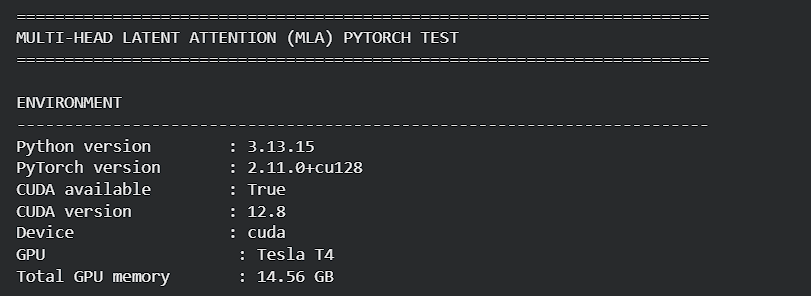
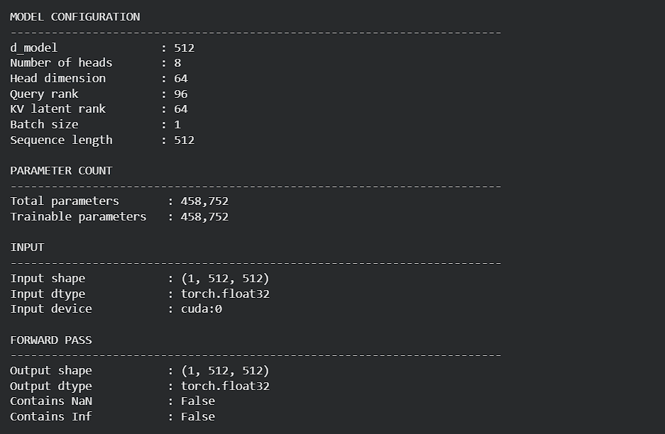
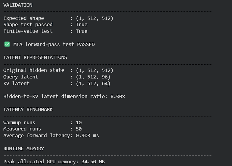
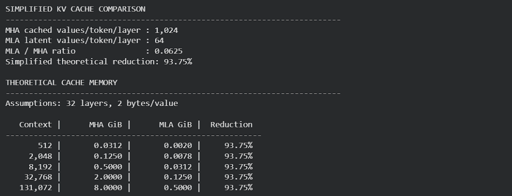
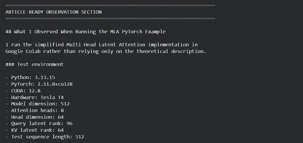
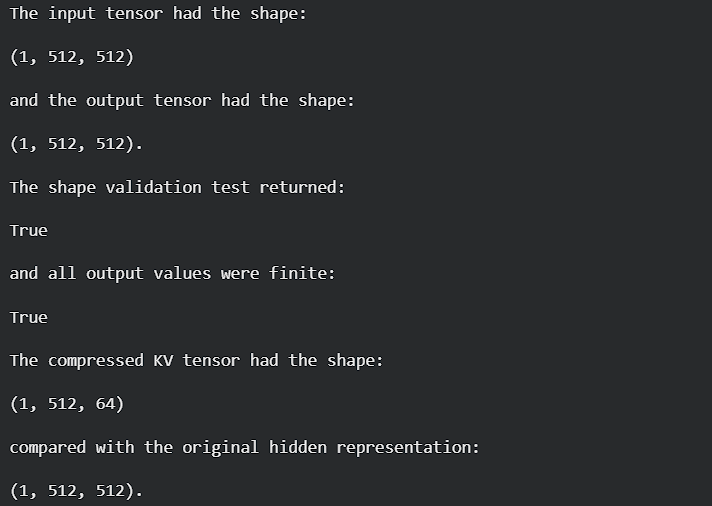
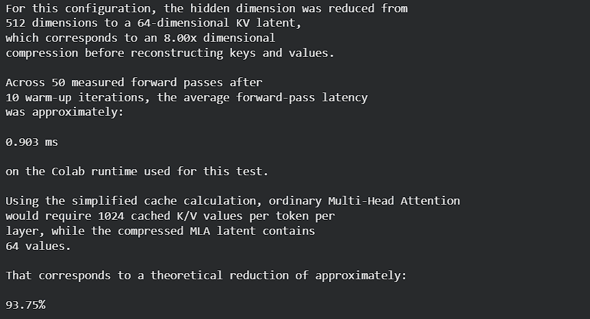
for the compressed latent portion of this educational example. This number should not be interpreted as the exact memory reduction of DeepSeek’s production MLA implementation. Real MLA also includes a separate positional component for decoupled RoPE, and production systems use different cache layouts, data types, kernels and inference optimizations. The experiment nevertheless made the basic reason for MLA’s memory advantage concrete: instead of retaining independently expanded key and value representations for every attention head, the architecture can retain a much smaller learned latent representation.

✅ EXPERIMENT COMPLETED SUCCESSFULLY

Frequently asked questions about Multi-Head Latent Attention

What is Multi-Head Latent Attention?

Multi-Head Latent Attention is an attention architecture introduced with DeepSeek-V2. Instead of caching full per-head keys and values for every previous token, MLA uses low-rank joint compression so that much of the required information can be stored in a smaller latent representation.

What does MLA stand for in DeepSeek?

MLA stands for Multi-Head Latent Attention.

Who introduced Multi-Head Latent Attention?

MLA was introduced by DeepSeek in the DeepSeek-V2 architecture published in 2024.

Does DeepSeek-V3 use MLA?

Yes. The DeepSeek-V3 technical report states that the model uses Multi-Head Latent Attention together with its DeepSeekMoE architecture.

Why does MLA reduce KV-cache memory?

Standard MHA stores expanded key and value representations for every attention head. MLA instead caches a substantially lower-dimensional joint KV latent plus the positional information required by its decoupled RoPE mechanism.

Is MLA the same as Multi-Query Attention?

No. MQA reduces cache memory by sharing one key/value head across many query heads. MLA uses learned low-rank compression to create a latent representation from which key/value information is obtained.

Is MLA the same as Grouped-Query Attention?

No. GQA shares KV heads between groups of query heads. MLA compresses KV information into a low-dimensional latent representation.

Does MLA reduce attention complexity from O(n²)?

Not by itself. MLA primarily reduces KV-cache storage and associated memory traffic. Other methods are required to fundamentally change full attention’s sequence-length scaling.

Can I implement Multi-Head Latent Attention in PyTorch?

Yes. The low-rank architecture can be implemented using ordinary PyTorch linear layers and attention operations. A production implementation additionally needs efficient caching, decoupled RoPE, absorbed projections and optimized kernels.

What is FlashMLA?

FlashMLA is DeepSeek’s optimized kernel project for executing Multi-Head Latent Attention efficiently on supported GPU hardware. It is an implementation optimization rather than a different attention architecture.

For primary sources, read the DeepSeek-V2 paper on arXiv, the DeepSeek-V3 technical report, the DeepSeek-V3 GitHub repository, and the FlashMLA GitHub repository. For related GenAITrail reading, see GLM-5.3 explained and GLM-5.3 costs and benchmarks.

Final takeaway

Multi-Head Latent Attention is best understood as a change in what a transformer considers worth remembering during generation.

Conventional Multi-Head Attention remembers fully expanded key and value vectors for every attention head.

MLA learns a smaller latent representation instead.

The architecture then separates position-sensitive information through decoupled RoPE and reorganizes projection matrices so that efficient inference does not necessarily require reconstructing conventional K/V tensors.

That distinction is important.

MLA is not simply:

“MHA with smaller keys.”

It is a coordinated design involving low-rank KV compression, positional separation, learned reconstruction and inference-time matrix absorption.

For short-context models, this may sound like another attention variant.

For long-context LLM serving, where gigabytes of GPU memory can disappear into KV caches, it addresses one of the most practical limitations of autoregressive transformers.

And that is the real DeepSeek reason Multi-Head Latent Attention has received so much attention since DeepSeek-V2: it connects an architectural idea directly to the economics of running large language models.

Multi-Head Latent Attention (MLA) Explained: DeepSeek Architecture, KV Cache, Math & PyTorch Code